Simulating the wind in an empty EFV
Simulating the
wind in an empty EFV by Victor Reijs
is licensed under CC BY-NC-SA 4.0


Introduction
One of the recommendatiosn of Blocken [Blocken, 2015], to verify
CFD, is to determine the homogeneity of an empty Flow
Volume (aka windtunnel). There are two situations that are
imortant:
- one where we have one type of ground layer with a roughness
height ks (as elobared below),
- and one to have two or more grounds layers with different
roughness heights in a CFD model.
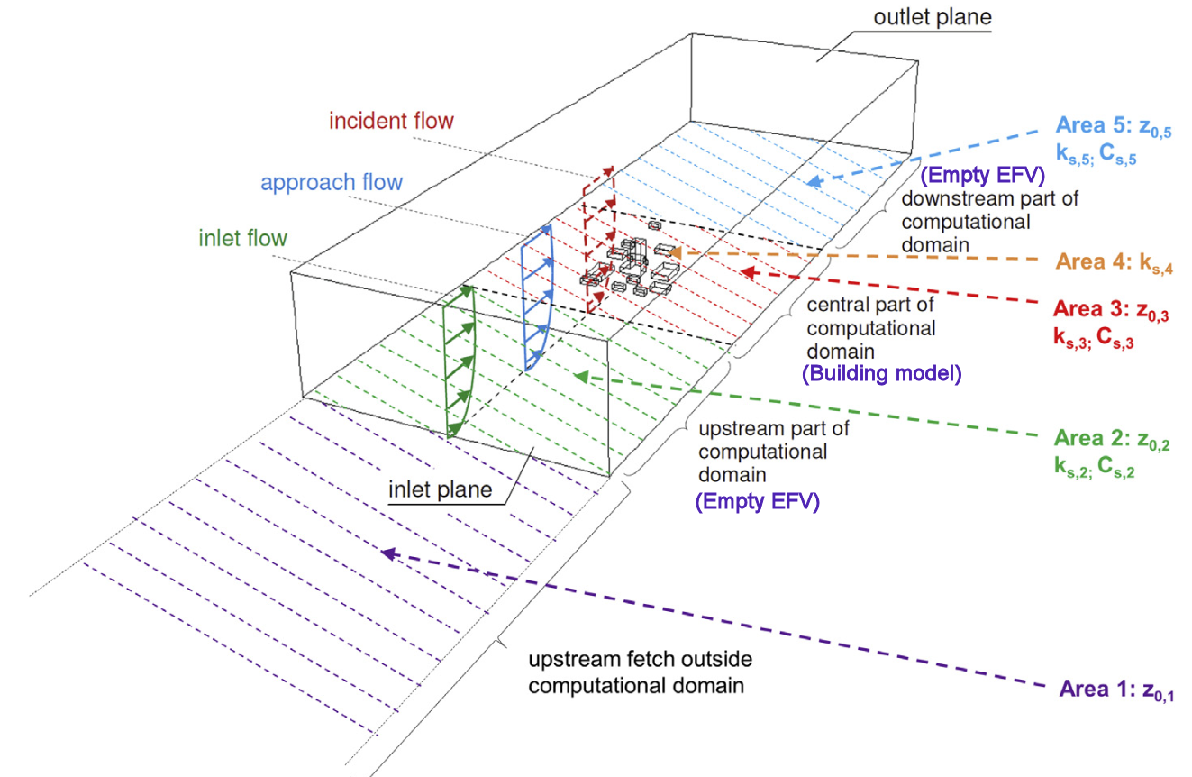
On this web page a simulation of an empty External Flow Volume (EFV)
with one ground layer, to determine horizontal homogeneity of domain
[Blocken, 2007, 2015]) is documented. The inlet ABL is kept
constant, while the ground ks is varied.
These CFD tips are
being used.
This web page has the followig sections:
Bold purple text needs attention.
Working in SketchUp
- Include at the back (100m from point zero) a small (dummy) box
(which is needed for being able to simulate things in CFD as an
empty EFV space is being simulated)
- If finished: 'Save' en 'Download' -> 'STL'
- Effort: 0.25 hours
Editing 3D-model in SIMSCALE
The following steps are done:
- Import het STL
model
- Edit this model by: Edit a copy
- Make a Flow Volume -> 'External flow volume'.
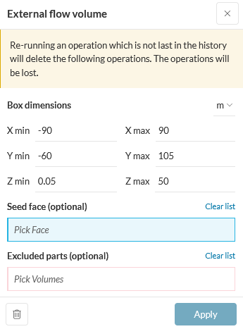
- Delete the dummy box
- Save
- Effort: 0.25 hours
Configuring the CFD
The model is at Empty Flow Volume,
SIMULATIONS: EFV; Simulation Runs:
RH=5.44,Cs=0.9,MS=0.3,CB2, RH=0.0544,Cs=0.9,MS=0.3,CB2 and
RH=544,Cs=0.9,MS=0.3,CB2.
The following steps were taken to derive the above Simulation
Runs (based on
CFD tips):
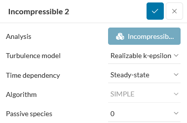
- Goto SIMULATIONS +
- Incompressible -> Turbulence-model -> Realizable
k-epsilon [Franke, 2007, page 14] [Franke, 2007, section
B.2.1 for PWC]
- Materials -> Air -> Apply
Assigned Volumes -> Flow region
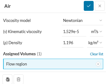
Remark: this is not the recommended temperature related air
parameters as in CFD tips. The above looks to be close to 22C
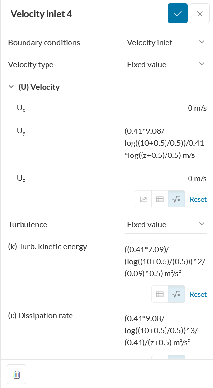
- Boundary conditions
- Velocity Inlet
Assigned Faces -> the wind side
(U) Velocity -> Uy -> ABL Formula
(9.08m/sec at 10m and z0=0.5m, the wind direction
is 180deg [S])
(0.41*9.08/log((10+0.5)/0.5))/0.41*log((z+0.5)/0.5)
Turbulence -> Fixed value
(k) Turb. kinetic energy -> ABL derived Formula
(0.41*7.09/log((10+0.5)/0.5))/(0.41*(0.09)^0.5)*1/(z+0.5)
<an error: the 7.09 should have been 9.08!>
Remark: next time need to
change this.
(ε) Dissipation rate -> ABL derived Formula
(0.41*9.08/log((10+0.5)/0.5))^3/(0.41)/(z+0.5)
Save
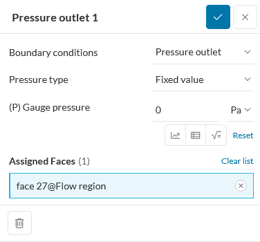
- Pressure outlet
Assigned Faces -> opposite inlet side
Save
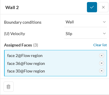
- Wall
Assigned Faces -> two sides and top
(U) Velocity -> Slip
Save
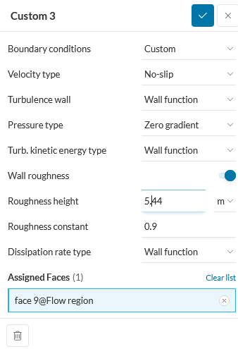
- Custom (ground)
Assigned Faces -> bottom side
Wall roughness -> On
Roughness height -> 5.44m (kS; 5.44m
(~11*z0), [Blocken, 2015, formula (15)]. as
SIMSCALE is based on OPENFOAM and Cs=0.9).
To see the influence: also a kS; 0.0544 and kS;
544 are tested
Roughness constant -> 0.9 (Cs)
Save
- General Mesh
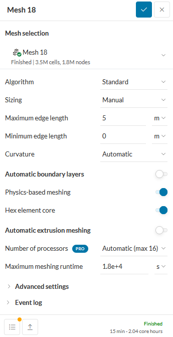
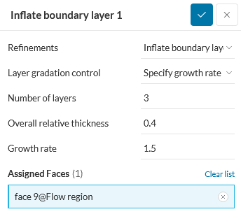
- Mesh -> Refinements -> Inflate boundary layer
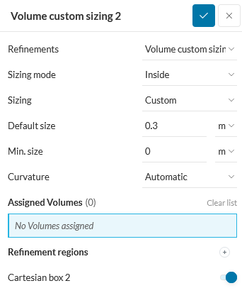
- Mesh -> Refinements -> Volume custom sizing
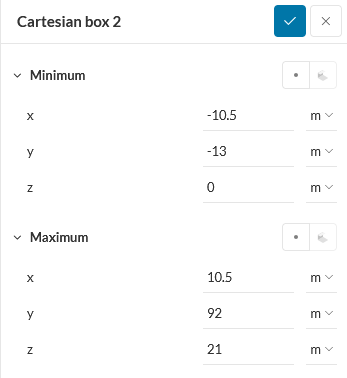
- Mesh -> Geometry
primitives
- Effort: 0.5 hour
Running the CFD
- Simulation Runs +
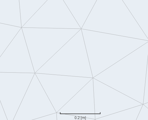
- Resulting Mesh size (specified=0.3m) in the Cartesian box
2 (actually around 0.2m):
Outside this Cartesian box 2 the actual Mesh size is
around 4m.
If no Cartesian box 2 was present, the overal actual
Mesh size was 0.5m.
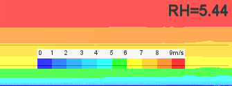
- Results of simulation:
The inlet ABL has in all cases an z0=0.5m.
Remark: Screenshots
in SIMSCALE do not seem to be properly coloured!
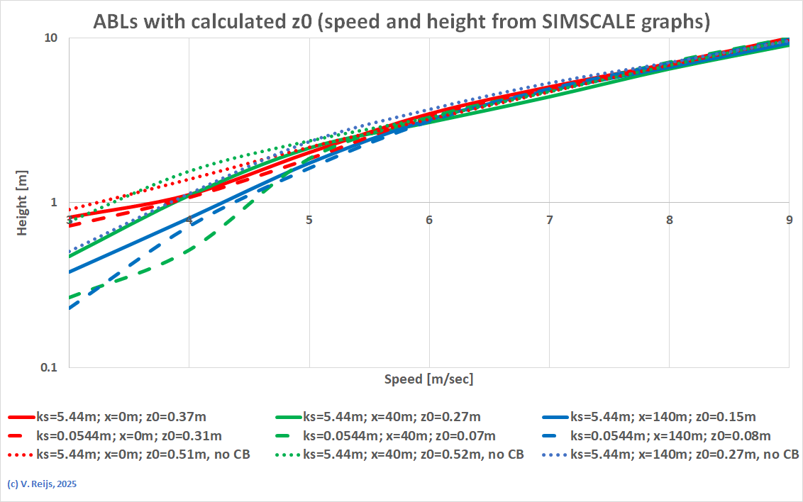
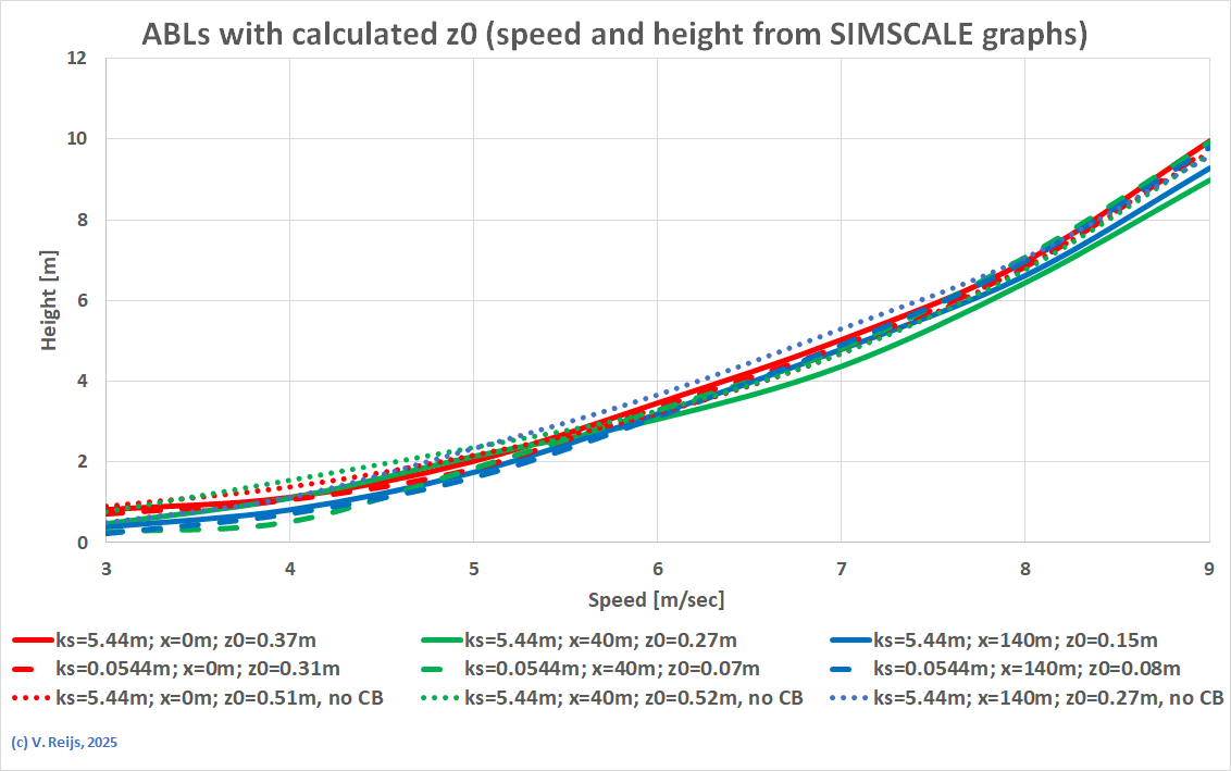
- With the speed at certain heights,
one can calculate the equivalent z0, this has been
done for the situation with Cartesian box 2 with ks=5.44m
(a calculated equivalent with z0=0.5m), ks=0.0544m
(a calculated equivalent with z0=0.005m); and without
the Cartesian Box 2: ks=5.44m (a calculated
equivalent with z0=0.5m).
Logarithmic height:
Lineair height:
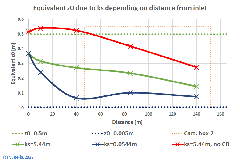
- Here is a view how the equivalent z0
depends on the distance from inlet (the inlet ABL has a z0=0.5m,
the windtunnel is 165m long).
Green cruve: ks=5.44m with Cartesian box 2;
blue curve: ks=0.0544m with Cartesian box 2;
Red curve: ks=5.44m without Cartesian box 2
:
 .
.
For the red curve: The ks of the ground-layer is
5.44m and Cs=0.9 (calculated equivaleny z0=0.5m),
the inlet ABL is z0=0.5m and actual mesh
size is everywhere ~0.5m; the measured equivalent z0
decreases. As ground and ABL are 'matching', I would expect
that the equivalent z0 would stay close to 0.5m.
For the green curve: For ks of the ground-layer
is 5.44m and Cs=0.9 (calculated equivalent z0=0.5m)
and actual mesh size in the Cartesian box 2 is 0.2m and for
the rest 4m; the measured equivalent z0 looks to
decrease considerable.
For the blue curve: For ks of the ground-layer is
0.0544m and Cs=0.9 (calculated equivalent z0=0.005m)
and actual mesh size in the Cartesian box 2 is 0.2m and for
the rest 4m; the measured equivalent z0 is almost
a factor 10 higher. This could be because the inlet ABL z0
is high (0.5m) compared to the ground-layer's.
Remark: Is the found difference
between ks and equivalent z0
significant?
- A full length overview, with horizontal homogenity:
- kS= 5.44m
The full 165m:

The last 17m (starting at 140m; black horizontal lines at 3.4
and 6.8m):
A quiet constant velocity of 7.9m/sec@6.8m
- Some possible reason why this is all not functioning as
expected:
- This is related to the three areas of ks+
[Brocken, 2007, section 4.1] or y+ in SIMSCALE.
- And note this from
an ANSYS manual: "that it is not physically
meaningful to have a mesh size such that the wall-adjacent
cell is smaller than the roughness height. For best
results, make sure that the distance from the wall to the
centroid of the wall-adjacent cell [yp] is
greater than ks."
In Blocken [2007, sect. Summary and conclusions]
is told that in 2007 no code was available to overcome this
restriction of yp>ks.
Remark: SIMSCALE's
documentation also refers to the restriction yp>ks.
- How to deal with this restriction, the
thinking is as follows:
Remark: Not sure if below idea is
correct
- for the entire volume outside the 3D model
(areas 2, 3 and 5): use a ksrond (10.9*z0)
and Cs=0.9 (there are no obstacles).
The mesh size outside the 3D model volume should be 2*ksrond
using a properly defined inflate boundary (min. 3 layers).
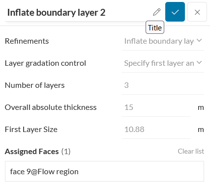
Here is an example Inflate boundary layer (for a z0=0.5m
-> ksrond = 5.44m): Number of layers: 3;
First Layer (mesh) and absolute thickness = 2*ksrond
= 10.88m:
And above this inflate boundary; a mesh size of say 0.5m.
If using this with the general mesh size of 1m, this Inflate
boundary layer does not do anything.
If increasing the general mesh to 11m;
the Inflate boundary is working as configured, but no
Horizontally homogeneous of the ABL (also z0=0.5m)
is happening (in the first 10m from the Inlet a
step is happening):
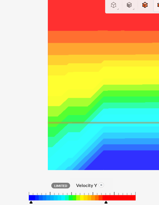
So this exercise is not very succesful...
Also tried to reduce k (turbulent kinetic energy) with a
factor of 4 (as proposed by Blocken [2007, section 7.1.e).
Kept all the same as above with the 11m mesh size. No
influence.
- for the ground within the 3D model (area 4): use
a ks3d of say ksrond /10 (Cs=0.9).
The explicit obstacles in the 3D model will define the
actual roughness (maybe one even don't need to explictly
define the roughness height for this 3D model volume). For
this ground; use inflate boundary (min. 3 layers) and an
overall 3D model volume mesh size of say 0.5m or smaller.
- and one should pay attention to the transition between the
two mesh sizes of the volumes (aka no discontinuity in speed
due to different mesh sizes).
- sdas das
- Effort: 0.5 human hours and 7 CPU hours per kS
Conclusions
- The influence of kS looks to be:
References
Blocken, Bert et al.: CFD simulation of the
atmospheric boundary layer: wall function problems. In:
Atmospheric Environment 41 (2007), issue 3, pp. 238-252.
Blocken, Bert: Computational Fluid
Dynamics for urban physics: Importance, scales, possibilities,
limitations and ten tips and tricks towards accurate and reliable
simulations. In: Building and Environment 91 (2015), pp.
219-245.
Franke, Jörg et al. COST Action 732: Best
practice guideline for the CFD simulation of flows in the urban
environment. Brussels, COST Office 2007.
Wieringa, Jon and R. Agterberg: Mesoscale terrain roughness
mapping of the Netherlands. In: TR-115 (1989).
Acknowledgements
I would like to thank people, such as Ezra van de Elst, Frank van Gool, SIMSCALE
Support and others for their help, encouragement and/or
constructive feedback. Any remaining errors in methodology or
results are my responsibility of course!!! If you want to
provide constructive feedback, please let me know.
Major content related
changes: December, 21, 2024
-90