CFD tips for a traditional windmill environment
CFD tips for a traditional windmill
environment by Victor Reijs
is licensed under CC BY-NC-SA 4.0


Introduction
This page gives some requirements how to configure one's own CFD
simulation. It is built around the 10 tips of Blocken [2015] and
feedback from others.
There is a slight bias for SimScale (based on OpenFOAM) in these
tips (but it is written in such a way that one can figure it out for
other CFD software).
Several questions are
outstanding, see below purple text. If you have input, please
let me know.
The wind mill environment
On this web page we will be looking at a traditional wind mill
(normally a diameter of ~7m, height of ~25m and sails span of ~22m;
there are of course many variations;-) in a urban environment
(although a more pastoral environment migth also be the case). So
not many high buldings around (say up to 12m high) and hopefully
also no high trees (say an z0 around 0.5 to 1m), but the
build and green environment can be changing. And here CFD will be
helpful to simulate the influence of new buildings and/or growing
trees.
At present a circle with a radius of 400m around the mill is chosen
to evaluate the wind mill biotope (Influence circle). This will also
be proposed for the CFD simulation.
An anemometer could be placed on/near the wind mill to record wind
speed/direction. The space for the rotating sails is of importance
as this will provide an impression of the available power.
The space for the rotating sails could be evaluted using Rotating Zone, but no experience yet has been gained on this.
Requirements
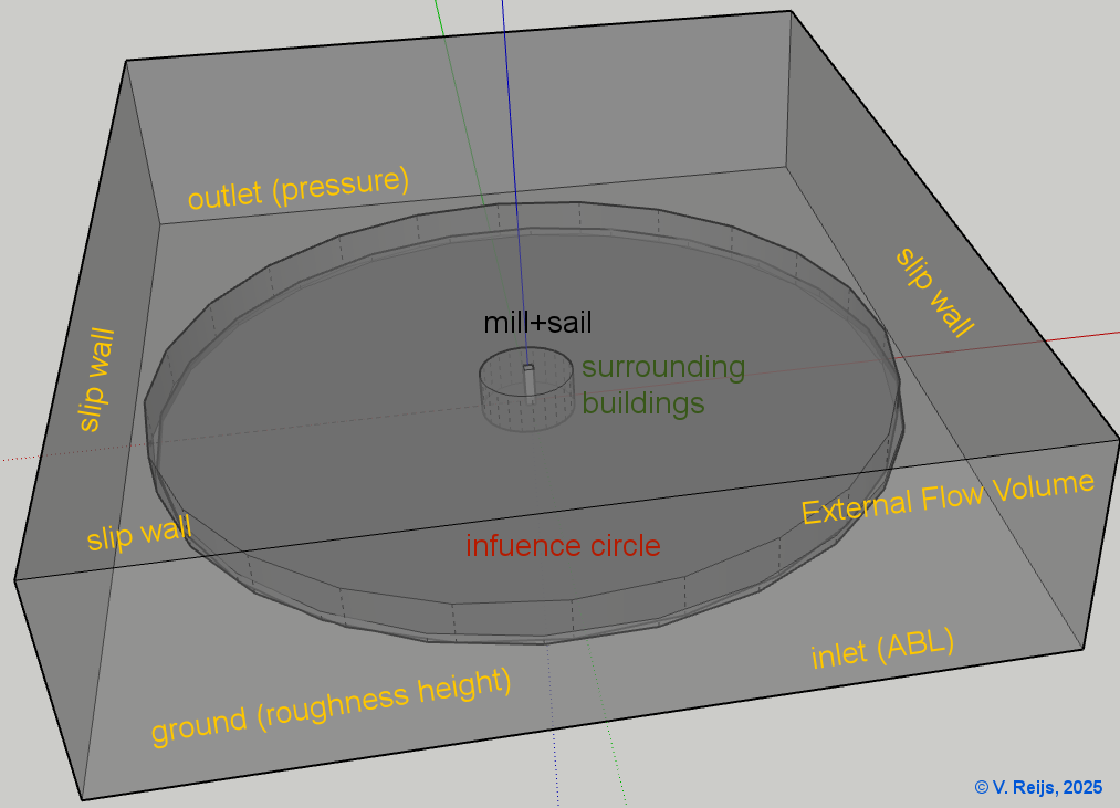
Building model
Some six different regions can be defined (between square
brackets, the location
and recommended grid size):
- Buidling model
- Functional spaces (e.g. the space for the rotating sails
[radius 15m and thickness 1m] or location of an anemometer
above the cap [4*4*4m]): [1 ->
0.3m]
- Mill (building of interest) (say radius 15m [sail length],
height 45m [mill cap height + sail length]): [2 -> 0.75m]
- Surrounding buildings (radius of 50m): [3 -> 1m]
- Influence circle (radius of 400m): lowest 10m has [4 ->1], rest [5 -> 2.5m]
- All regions have a height of mill cap height + sail length
- Empty External Flow Volume (EFV)
The Building model will be rotated (in model editing mode) to
simulate changing wind direction. If the CFD software supports PWC
[Pedestrian Wind Comfort), the rotation will be done within the
CFD machine.
CFD External Flow Volume (EFV)
There are two types of guidelines that need
to be obeyed when looking at the described wind mill environment
(EFV or windtunnel):
- Minimum distances (assumming the wind mill is in the
middle of the Influence circle) between the Building model
and the surfaces of the EFV (domain):
- Make sure that any building is at least 5*Hbuilding
from the lateral (Xmin and Ymin), inlet (Ymin)
surfaces of the EFV [Franke, 2007, page 18].
- Make sure that any building is at least 15*Hbuilding
from the outlet (Ymax) of the EFV [Franke, 2007, page
18].
- Ground: Zmin: height minimum = 0.05m (to overcome
model rounding errors [gaps]).
- Blocking ratio (Hmax is height of the highest
building; if Hmax is height of the mill cap height
then add the sail length to Hmax):
- Height EFV (Zmax): Hdomain>6*Hmax
[Franke, 2007, page 17]
- Blocking ratio: Adomain>3*Abuilding
[Gool, 2025, pers. comm & Blocken, 2015, formula 12]
Turbulence model
CFD solver must have minimum capability of solving the Navier-Stokes
fluid flow equations for a three-dimensional incompressible flow
analysis of steady state [Green Mark Department, 20016,
section A2].
RANS is being used and this provides a time-averaged stream. This
provides relative good results for wind velocities used for
turning/operating traditional wind mills (>2.5Bft).
Allowable turbulence models: one-equation Spalart-Allmaras model,
the standard k-ε model and its many modified versions, such
as the Renormalization Group (RNG) k-ε model and the realizable
k-ε model, the standard k-omega model and the k-omega
shear stress transport (SST) model [Blocken, 2015, page 229].
Recommendation: minimally standard k-ε model,
while RNG and realizable k-ε model provide good
solutions for an PWC (high Re number) environment (assuming that a
mill is a tall person;-) [Gool, 2025, pers. comm.] and [Franke,
2007, section B.2.1 for PWC].
URF’s [Under Relaxation Factor]: P=0.30, U=0.7, k=0.6, ω=0.6 (pers.
comm, Gool, 2025).
With k is:
k=((0.41*Uhref)/(ln((href+z0)/(z0))))^2/(0.09)^0.5 [m2/sec2]
with href normally 10m
With epsilon is:
epsilon=((0.41*Uhref)/ln((href+z0)/(z0)))^3/(0.41)/(z+z0) [1/sec]
with href normally 10m
LBM solvers would allow
a good time vayring solution of the wind mill environment.
No experience has been gained yet with this.
Atmosphere conditions
Temperature
Isothermal condition at 15°C air temperature [ISA 1976] at steady
state condition:
Kinematic viscosity:
1.50e-5 m2/sec
Density: 1.23
kg/m3
Atmospheric Boundary Layer [ABL]
The equations for the inlet ABL can be found at Blocken [2015,
section 5.4] (see also at SimScale).
A windspeed of 5m/sec@10m is taken.
Remember that the z0 can be different for different wind
directions (as it depends on the roughness of the wind [upstream
from the flow region] from that direction). The (average) wind speed
varies also with the wind direction.
Recommendation: use formula as given by SimScale.
It looks that OpenFOAM is not able to handle a high k (like 1.072),
so proposed to use 0.375 m2/sec2 [pers. comm.
van der Elst, 2025]..
A quality mesh grid
Using the earlier
described regions (without the functional space[s]), the
areas of different meshing sizes are depicted here:
Some recommendations by Green Mark Department [2017, section A5]
and Blocken [2015, page 232-233]:
- Recommended grid sizes:
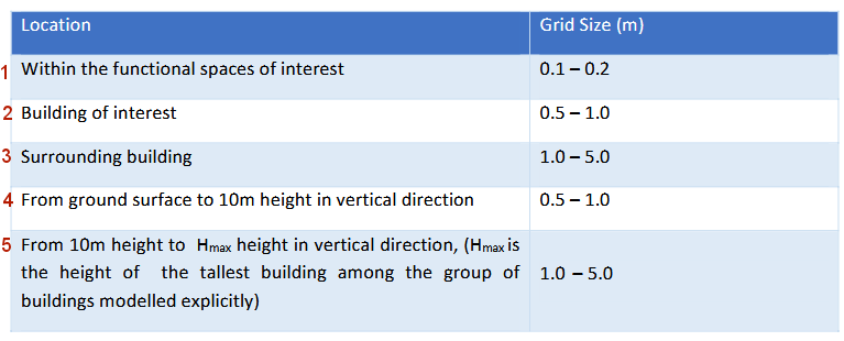
- cell skewness <0.9
- Stretching ratio or Aspect Ratio <1.3
- Hexahedral cells are preferred (for instance Hex-dominant
setting in SimScale) over tetrahedral cells
- No tetrahedral cells at walls
- 10 cells per cube root of the building volume (minimum 3 cells
per direction)
- minumum 4 cells between every two buildings [2025, pers. comm.
Gool], otherwise merge the buildings [2025, pers. comm. Gool]
- A functional space or evaluation height should be at least in
3rd grid cell from ground.
- The mesh grid yg should be
larger than 2*ks
[SimScale and Blocken, 2007, section 6 and
7].
- create a gradual change in mesh sizes (to overcome volume
transition discountinuities; a volume transition of on average 4
or max. 5 [Wimshurst, 2022]);
which is a distance transition of average 1.6. This needs to
be matched also with the top layer of the boundary layer!
Others (e.g. SimScale ):
- make sure the mesh quality metrics
(Orthogonality<88; Edge Ratio<100; Volume Ratio<100;
Aspect Ratio<100; Tetrahedral Aspect Ratio [preferable]=0;
Skewness<100) are within boundaries
A grid
convergence study is recommended if no previous experience
has been gained.
<In the future an example of a bad
and good mesh will be presented on this page>
The roughness parameters
There are two types of roughness specifications:
- aerodynamic roughness length z0
This is used e.g. in the
ABL.
- equivalent sand-grain roughness height ks
ks is modelling height roughness for surfaces (in SimScale for ground
(non-slip wall))
There is the Roughness constant (Cs) (between
uniform (0.5) and strongly non-uniform (1) roughness height). A
common value for Cs looks to be 0.9 as quoted from
Blocken by Townsend [2024, page 2], but other values are
possible [Townsend, section 3].
For software based on OpenFOAM (such as
SimScale) and ANSYS/Fluent, the conversion between z0,
ks and Cs is:
ks~9.8*z0/Cs and using Cs=0.9
gives ks~10.9*z0
For ANSYS-CFX based software, the conversion between z0
and ks is:
ks=29.6*z0 (as it has an implicit/fixed Cs=0.33)
The mesh grid size yg should be
around ks (yg>2*ks and yg=2*yp).
A mesh grid size of yg of 1 to 5m (Surrounding buildings)
looks to be minimumly needed, and that would result in a ks
of 0.67m to 3.33m or a z0 of around 0.07m to 0.33m.
Thus a roughness height modelling could be done for an Open
(z0 = 0.03m) to Rough environment (z0
= 0.25m), all other environments with a higher roughness
length z0 should be modelled using explicit 3D boxes
[Blocken, 2007, section 7.1(b)].
An example how this is done can be seen in this picture [Chen,
2022, Figure 1]:
Different roughness araes
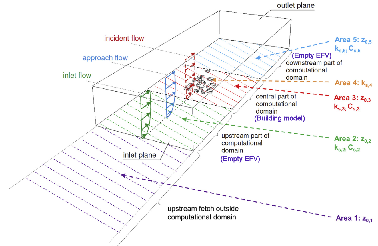
Figure 16 of Blocken [2015].
In SimScale:
- Area 1: impleciet by ABL
- Area 2, 3, 4 and 5: governed by roughness height (ks-x)
and roughness constant (Cs). See for relation between
z0, ks and Cs here. Best values
for ks; if
z0 is not too large:
- ks,2: related to inlet z0
- ks,3: related to inlet z0: ks,3=ks,2
- ks,4: related to an z0 < 0.1m, or
let say ks,4<ks,2/10. This ks,4
can be small as the modelled obstacles will determine the real
roughness.
- ks,5: related to inlet z0: ks,5=ks,2
Also check that the stream is reacting properly to changing ks.
Remark: Still need to find out how to
make several areas of different Roughness height ks
and Cs for the EFV in SimScale. This needs to be done in the CAD program:
SketchUp is not able to do this: Better to use OnShape. For
now: for all areas 2, 3, 4 and 5 the same (z0,) ks-x
and Cs are used.
Horizontal homogeneity of empty
computational domain
When one removes all objects (but keep roughness heights/lengths
as wanted), a horizontal homogeneity in speed and turbulent
kinetic energy should be achieved.
Is horizontal homogeneity also needed for
turbulent kinetic energy?
And example is here (-13.6m to 68m):
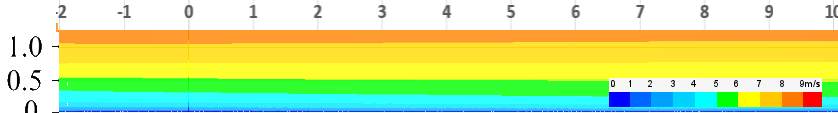
Also check that the stream is reacting properly to changing ks.
Higher-order discretization schemes
Don't use 1st order gradient schemes; 2nd
order (such as Gauss) should be ok.
SimScale uses default
Gaussian integration.
Evaluation of convergence
Check in the convergence plots if the solution converges smoothly
and converges to a stable end (so no oscillations). Termination
threshold (for for instance pressure) preferrable around 10-3.
Recommendation: Check in SimScale: Simulation Runs ->
Convergence plot -> Residuals
Grid convergence study
The mesh grid resolution should be varied using
a linear refinement factor of at least 1.26 in each direction (so
that is around 2 [~1.263] for 3 directions). The
results should not change significantly. At least three
refinements checks need to be done (reduce and increase the recommended grid
sizes with factor of 1.26).
What do we measure
Wind speed (perpendicular to the plane of the sails: at eight
locations [long and short rest positions] at 3/4 of the sail
length), the turbulence intensity (TI), y+ (according to SimScale; but I have not seen
practical use for it in wind mill environment. If people have
ideas, let me know) and convergence plots.
Validating the results
One needs to validate the results using scientific articles.
Areas to be covered:
- study of non-CFD methodologies
Examples: DHM-formula,
ST workflow,
EJL workflow
- porous media to proxy trees: comparing CFD results with
published measurements in vivo
Examples: Nageli,
Ren, Tree proxies
- comparing CFD results with professionally made wind quality
reports around traditional wind mills (that use CFD or other
methodologies).
Examples: De
Hoop, Rijn en Lek
- comparing CFD with wind measurements at traditional wind
mills.
Examples: Impington,
Rijn en
Lek
- consult CFD experts.
See acknowledgements section on each web page
- keep critically reviewing the meshing sizing and CFD results.
Example: CFD tips,
open questions
Conclusions
If one compares two or more environments, the relative valuee become
important. If the aerodynamic system is relatively linear, all
unknown method parameters will be divided out, and thus the values
of these parameters become a little less important (again: as
long as we are in a linear environment)!
<Can only provide text for this section when things are fully
understood, reviewed and tried>
References
Blocken, Bert et al.: Modification of
pedestrian wind comfort in the Silvertop Tower passages by an
automatic control system. In: Journal of Wind Engineering
and Industrial Aerodynamics 92 (2004), pp. 849-873.
Blocken, Bert et al.: CFD simulation of the
atmospheric boundary layer:wall function problems. In:
Atmospheric Environment 41 (2007), issue 3, pp. 238-252.
Blocken, Bert: Computational Fluid
Dynamics for urban physics: Importance, scales, possibilities,
limitations and ten tips and tricks towards accurate and
reliable simulations. In: Building and Environment 91
(2015), pp. 219-245.
Chen, Zhaoqing et al.: Numerical simulation of Atmospheric
Boundary Layer turbulence in a wind tunnel based on a hybrid
method. In: Atmosphere 13 (2022), issue 12.
Franke, Jörg et al. COST Action 732: Best
practice guideline for the CFD simulation of flows in the urban
environment. Brussels, COST Office 2007.
Green Mark Department: BCA GREEN MARK FOR
RESIDENTIAL BUILDINGS: Technical guide and requirements. In:
(2017), issue GM RB: 2016.
Townsend, Jamie, F. et al.: Roughness constant
selection for atmospheric boundary layer simulations using a k-ω
SST turbulence model within a commercial CFD solver. In:
Advances in Wind Engineering 100005 (2024), pp. 1-10.
Winshurst, Aidan: Sizing inflation layers
using a y+ estimation tool. In: (2022).
Winshurst, Aidan: Fluid mechanics 101:
Calculators & tools. In: (2025).
Acknowledgements
I would like to thank people, such as Frank van Gool, Ezra van
de Elst, SimScale Support and others for their help,
encouragement and/or constructive feedback. Any remaining errors
in methodology or results are my responsibility of course!!! If
you want to provide constructive feedback, please let me know.
Major content related
changes: January 8, 2025