HomeUpSearchMail
NEW

Simulating the wind around a house

Simulating the wind around a house by Victor Reijs is licensed under CC BY-NC-SA 4.0

Introduction

• Working in SketchUp
  
• Editing 3D-model in SIMSCALE
• Configuring the CFD
  
• Running the CFD
  
• Conclusions
• References
• Acknowledgements

Bold purple text needs attention.

Working in SketchUp

• Made a house of 10*10*9m (l*w*h). Included in the house height can have a gable roof of 4m.
• The length of the house ranges from y=0m to y=10m.
  
• The width of the house ranges from x=-5m to x=5m.

• block	wind against gable	wind along gable

  
  
• If finished: 'Save' en 'Download' -> 'STL'
• Effort: 0.5 hours
  

Editing 3D-model in SIMSCALE

• Import het STL model
• Edit this model by: Edit a copy
  
• Make a Flow Volume -> 'External flow volume'.
  
  
• Delete the house
  
• Save
• Effort: 0.25 hours

Configuring the CFD

The model is at House.
The following steps were taken to derive the above Simulation Runs (based on CFD tips):

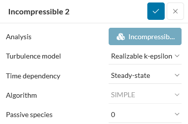
• Goto SIMULATIONS +
• Incompressible -> Turbulence-model -> Realizable k-epsilon [Franke, 2007, page 14] [Franke, 2007, section B.2.1 for PWC]
  
  
• Materials -> Air -> Apply
  Assigned Volumes -> Flow region
  
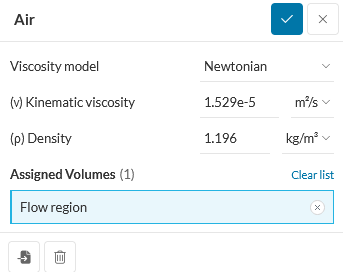
  Remark: this is not the recommended temperature related air parameters as in CFD tips. The above looks to be close to 22C
  
• Boundary conditions
• Velocity Inlet
  Assigned Faces -> the wind side
  (U) Velocity -> U_y -> ABL Formula (7.09m/sec at 10m and z₀=0.03m, the wind direction is 180deg [S])
  (0.41*7.09/log((10+0.03)/0.03))/0.41*log((z+0.03)/0.03)
  
  Turbulence -> Fixed value
  (k) Turb. kinetic energy -> ABL derived Formula
  ((0.41*7.09)/(log((10+0.03)/(0.03)))^2/(0.09)^0.5)
  
  (ε) Dissipation rate -> ABL derived Formula
  (0.41*7.09/log((10+0.03)/0.03))^3/(0.41)/(z+0.03)
  
  Also z₀ of 0.03m and 2m are being tested.
  Save
  
  
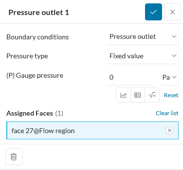
• Pressure outlet
  Assigned Faces -> opposite inlet side
  Save
  
  
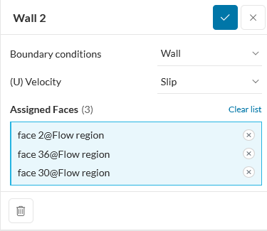
• Wall
  Assigned Faces -> two sides and top
  (U) Velocity -> Slip
  Save
  
  
• Custom (ground)
  Assigned Faces -> bottom side
  Wall roughness -> On
  Roughness height -> 5.44m (k_S; 5.44m (~11*z₀), [Blocken, 2015, formula (15)]. as SIMSCALE is based on OpenFOAM and C_s=0.9).
  Also k_S of 0.333 and 21.76m are tested
  Remark: k_S should have been 0.33m
  Roughness constant -> 0.9 (C_s)
  Save
  
  
• Mesh
  
  The resulting mesh cell size is on average around 0.9m.
  
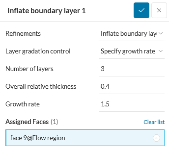
• Mesh -> Refinements -> Inflate boundary layer
  
• Effort: 0.5 hour per house type
  

Running the CFD

• Simulation Runs +
• Three house types have been simulated:
• a block house
• a house with gable roof, wind against the gable
  
• a house with gable rood, wind along gable
• The speed in the y-direction (same as wind direction) has been determined in the middle of the house (on the y-axis).
  
• A block house (z₀=0.5m, k_s=5.44m, and Inflate Boundary 0.4 relative thickness of 0.9m = 0.36m)
  
  There were some oscillations in the residues of the simulation.
  
• House with wind against gable roof (z₀=0.5m, k_s=5.44m, and Inflate Boundary 0.4 relative thickness of 0.9m = 0.36m)
  
• House with wind along gable (z₀=0.5m, k_s=5.44m, and Inflate Boundary 0.4 relative thickness of 0.9m = 0.36m)
  
• House with wind along gable (z₀=0.03m, k_s=0.333m, and Inflate Boundary 0.4 relative thickness of 0.9m = 0.36m)
  
• House with wind along and against gable (z₀=0.03m, k_s=0.33m, and First Layer (mesh) Size = 2*k_s = 0.66m)
  
  Wind along gable:
  
  
  Wind against gable:
  
• House with wind along gable (z₀=2m, k_s=21.76m, and Inflate Boundary 0.4 relative thichness of 0.9m = 0.36m). This k_s is too big; the roughness height modelling is not functioning well anymore:
  
• Effort: 0.5 human hours and some 11 CPU hours per house
  

Conclusions

• Nägeli measured the wind speeds behind a Dichte Wand a henge (H=2.2m, width of 11H, optical porosity of ~17.5%, and z_0m of 0.03m). One could compare these a little with the above results of house with wind 'along gable' (H=10m, width of 1H, optical poristy of 0%, and z₀ of 0.03m).
  
  With Nägeli: H=2.2m, thus 0.55m::0.25; 1.1m::0.5; 2.2m::1; 4.4m::2; 8.8m::4.
  
  As the house (10m) is less wide than the 25m henge one would expect a faster increase of the speed for the house.
  The dip seen in the curves happens closer to he end of the obstacle if it is less porous. The rest of the  curves' forms looks similar (exponential).
  Remark: Is this comparison/evaluation between Nägeli and simulation correct?
  
• The curve z/H=0.25 can be higher than the z/H=0.5 and 1 curves; this can be seen in this houses' experiment and in Nägeli's.
  
• For certain houses ('block' or high z₀) the speed at low heights (z/H = 0.25 and 0.5) are higher than the speed of the ABL inlet. Simultaions by others also show this effect.
• The difference in speedfactor between 'House, along gable' and 'House, against gable' is some 15% (looks to be regardless of z₀).
  
• After a house: Some kind of compression towards the ground or increase of Turbulent Kinetic Energy (TKE below is of the House with wind along gable [z0=2m,]).
  
  The vertical line is at x/H=27.5, the lighter blue the more TKE.
  
• For some reason it was not possible to reduce the mesh size further than 0.9m (due to having not enough memory or resources). This could provide problems when looking at the absolute values, but hopefully one can compare the outcomes at some level.
  Remark: someone else will need to check these house configurations with smaller mesh size; with the aim to verify the results on this page.
  
• There is some residual instability for the House 'block'. The other houses look ok-ish.
  
• The influence of looking at wind speed magnitude instead of using windspeed(y) (same as inlet wind direction) is very small, except near the house.
• The 'block' house and 'along gable roof' are similar. This could be because the wind speed has been determined in the middle of the house; along y-axis (where block and gable have the same physical height).
• As it is not really known how a roof will be aligned with the wind (depending on direction of wind and positioning of the house); it is expected that the behavior of the roofed house will be between 'against gable roof' and 'along gable roof'.
  
• As expected, the lower the z₀ the longer it takes before the speed is back to the inlet.
• If we assume no obstacles within the first 100m from the mill (in above graphs this is at 11H); the curves could be seen as exponential, but tending to be linear. If obstacles are within this 100m, the exponential aspect becomes certainly important.
  

References

Acknowledgements

Disclaimer and Copyright
HomeUpSearchMail