HomeUpSearchMail
NEW

Analyses of measurements on Late-Minoan buildings

In the article of Papathanassiou, Hoskin and Papadopoulou [1992] an overview is given of some 200 buildings in Armenoi (Crete, Greece, 35.32° N latitude and 24.47° E longitude) from between 1450 - 1190 BCE.
Due to the above time period of construction, these buildings are likely to have been build under the Mycenaean domination.
Tholos grvae 014 at Armenoi


Evaluation of error in azimuth and altitude of Hoskin's data

Hoskin ([2001], appendix A.1) provides in his appendix all the azimuths and apparent altitudes of these buildings (see below picture for the location of the Zones).

Zones of Armenoi
        complex 

Hoskin's azimuths Zone A, B and C

The azimuths have an error (1 sigma) of  less then 1°  (Hoskin [2001], page 219), the measurements were done with compass and it was assumed that there were no magnetic anomalies (limestone rock), this assumption looks to be correct.

Hoskin's altitudes Zone A and B

The following error analyses of Hoskin's altitude calculations due to parallax for Zone A and B can be done:
Zone A is some 200 meter long and is on average 1700 m from the horizon (TV mast), so the max. azimuth error is than 2*atan((200/4)/1700)=3.4°. The 1 sigma due to parallax is assumed 3 times smaller then the max., so around 1.1°. The parallax error in azimuth will translate in an error for determining the altitude from figure 6 (Papathanassiou [1992]). The max. slope in that figure is around 77.5° (near TV mast), where an 1° azimuth change gives a max. change of 0.4° in altitude. This value can be halved because we want to know the average change (so between max. and zero slope): thus 1 sigma in altitude will be: 0.2°.
In the below analysis the parallax has no significant effect, because at each zone the altitude and azimuth of the mountain top has been measured.

Hoskin's altitudes Zone C

It can be determined that the parallax for Zone C is some 5° in azimuth (taken the average distance to the ridge [2300 m] and the length of Zone C from Zone A/B [200 m]). Hoskin only compensated for 4° (Hoskin [2003], pers. comm.), the resultant apparent altitude error (0.1°) is though not much due to this parallax error.
In the below analysis the parallax has no significant effect, because at each zone the altitude and azimuth of the mountain top has been measured.

My own observations

I have done my own observations on some 65 tholi  in June 2004:
In the below figure you see included the measurements of Hoskin (Hoskin [2001], page 259-260):
Comparison of
        several measurements

A few observations from this comparison:

Data analysis

My data analysis is based on the following:
When analysing this data corpus (using an average latitude of 35.32° N, time period around 1320 BCE and corresponding obliquity (Thom [1971], page 15)), the following density graph of observed topocentric declination distribution is gotten (pink line):
Distribution of directions

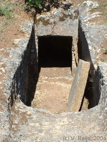
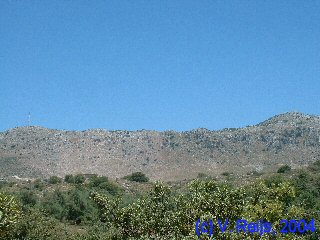
The above mentioned articles don't provide a detailed evaluation of what is visible in this distribution (except the general comment that the buildings were build in the general direction of sun/moon rise and/or aligned to a culturally  lunar related Mount Vrysinas). It is of course not easy to know what was meant some 3000 years ago, but the observed distribution could perhaps provide more info. Using Monte Carlo optimization a further study has been done.

Monte Carlo optimization

Because this set of buildings seems ideal for statistical analyses (in total  Zone ABCx has some 224 buildings, seemingly belonging to the same culture), it is perhaps possible to simulate the construction of these buildings with Monte Carlo optimization. It was tried with a set of some 4800 simulated constructions and several different clusters of dates to see if the observed curve could be approached.
Each cluster of dates tries to simulate a peak seen in the observed directions. A cluster of dates is assumed to be characterized by an average value (value close to the peak) and a variation around this (sigma in case of normal distribution). A date has been convered to a topocentric declination of the Sun.

To determine the optimum cluster of dates an optimizer is being used; the optimization solver of Excel does not work for this non-linear problem, so Evolver 4.0.5 and RISKOptimizer 1.0.8 has been used.
If one looks at the monuments for each individual zone one gets the following density graphs of the observed and expected (optimized) distributions when using an interval of 2º (close to the recommended value of 1.2º):
Graves in Zone A
Zone A
Graves in Zone B
Zone B
Graves in
              Zone C
Zone C
Graves in Zone C
Zone ABCx
Distribution differenc ebetween Expected and
              Observed
Comparing the Zone ABCx distribution functions of
expected and observed.

The above zones have the following optimized cluster of dates (the red values are calculated using Hoskin's original apparent altitude values):

Cluster of dates (between brackets the sigma) making the following peaks [Days]
Zone/number of graves peak4
peak3
peak2

peak1
peakA
peakB
peakC
peakD
A/109
11(13)
43(9)
61(6)
81(5)
NC
NC
NC
NC
B/52
NC
NC
NC
NC
95(9)
120(19)
NC
149(3)
C/59
NC
NC
NC
NC
95(3)
122(1)
131(2)
150(3)
ABCx/224
NC
NC
NC
61(4)
64(9)
82(4)
87(1)
96(5)
98(2)
121(1)
122(10)
132(2)
NC
NC

Legend

Statistical testing

The null hypothesis (H0) is:
The observed direction distribution of the graves is equal to the expected direction distribution resulting from the cluster of dates (determined by Monte Carlo).
for the following statistical tests:
  1. Chi-Square Goodness-of-Fit test
    The Monte Carlo optimization brings down the degrees of freedom (for Zone ABCx with c=20 and a k=28) for the Chi-square test (Kreyszig [1970], page 251, example 2 and this link [section: Critical Region]). Beside this, Yates' correction (using the definition from SPSS)  is needed, because some expected intervals are lower than 5.
    For Zone ABCx the observed directions look to be closely following the expected directions (X2=4, df=k-c=8; non-significant and thus keep H0).
  2. Kolmogorov-Smirnov Goodness-of-Fit test.
    The following condition from this link [section: Limitations of the K-S Test] limits the significance:
    "Perhaps the most serious limitation is that the distribution must be fully specified. That is, if location, scale, and shape parameters are estimated from the data, the critical region of the Kolmogorov-Smirnov test is no longer valid. It typically must be determined by simulation."
    Irregradless of the above, one still can state that the Kolmogorov-Smirnov test indicates that the distributional fit (see above graph) is acceptable (for Zone ABCx: D=0.032, N=224; non-significant and thus keep H0).
  3. The above has been done also with clusters of dates characterized by a uniform distribution (instead of normal distribution). No significantly different results were found; peaks have same value and the window width is around 2.8 sigma (which theoretically can be expected): the X2 and D are also comparable.
Because of the heavy dependency of the Monte Carlo optimization on the observed values (the cluster of dates has been derived from the observed values), the non-significance of the results looks correct. The graphs show also that the optimization, and thus the cluster of dates, could have been used in actual life when building the graves (the observed values).
Informed methods (like documents or other archaeological/ethnographic information) are needed to substantiate this in more detail.

If one further assumes that the equinoxes could have been used to pivot the festivals, one can determine the following cluster of dates for Zone ABCx (X2=12, df=14; again non-significant and thus keep H0): All of the above sigma includes the error of the measurements (sigma is 1°).

Why?

The above looks of course nice, but does this have any linkage to cultural or archaeological findings?
So I am looking for references to important festivals/myths/rituals/etc. occurring in the Minoan/Mycenaean culture and Crete region around 1320 BCE (using present day Gregorian calendar system):

These can be related of course with other events near the mentioned solar events, like stellar/lunar helical set and rise. If people have ideas on this, please let me know.

Stellar events

(as described in the Hesiod's Work and Days)

Here are a few stellar events (Aveni and Ammerman [2001], page 87-89) (these dates need to be checked, e.g. what calendar system is used: Julian or Gregorian!):
 

MFIRST ELAST EFIRST MLAST MHIGH EHIGH
Pleiades May 18rd March 23th


Betelgeuse July 7th


Sirius July 20th


Sep. 12th
Arcturus Sept. 4th
Feb. 18th


Orion's belt


Nov. 1st Sept. 4th
Spica
Oct. 2nd


Purple: Different than in article (but discussed with authors).

Topographical analysis

In the future a topographical analysis will be done of the local topography of the site, to see how the landscape could influence the distributed of directions.

Possible related rituals

I have asked people and got also some reactions. Here are a few:

Acknowledgments

I would like to thank the following people for their help and constructive feedback: Mary Blomberg, Alan Heckert, Göran Henriksson, Michael Hoskin, Richard Lowry, Jane McDonnell, Alun Salt, Bradley Schaefer, Doug Schwartz, Deborah Wilson and all other unmentioned people. Any remaining errors in methodology or results are my responsibility of course!!! If you want to provide constructive feedback, let me know.

Disclaimer and Copyright
HomeUpSearchMail

Last content related changes: Dec. 16, 2004