HomeUpSearchMail
NEW

Comparing Beljaars' method with CFD

Comparing Beljaars' method with CFD by Victor Reijs is licensed under CC BY-NC-SA 4.0

This is work in progress!!!

Introductie

• Informatie over de molen omgeving
  
• Eigenschappen van obstakels
• Maken 3D model in SketchUp
  
• Editing 3D model in SIMSCALE
• Configureren van de CFD
• Uitvoering van de CFD
• Conclusies
• Referenties
• Acknowledgements

Sorry for the two langauges gebruikt in deze webpagina!

Vette paarse tekst heeft nog extra aandacht nodig.

Informatie over de omgeving

• The ABL wind speed is logarithmic. Different z₀ will be used. Height of the obstacle is 2.2m and has a aerodynamic porosity of 8.5%. The velocity at 2.2m is 5m/sec.
  

  z0	H/z0	u@10m [m/sec]
  0.11	20	7.42
  0.0328	67	6.78
  0.0132	167	6.47
  0.066	333	6.3

  
  
• CFD wordt gedaan voor wind uit Zuid (180deg).
  

Eigenschappen van obstakel

• One box (fence) of 25m (Nägeli's fence) long, 40cm thick ad 2.2m heigh
  
• Nägeli fence, has an optical porosity of 20%; aerodynamic porosity 8.5% [Nägeli, 1953, Bild 2].
• 3D model of Nägeli's fence in SketchUp:
  
  

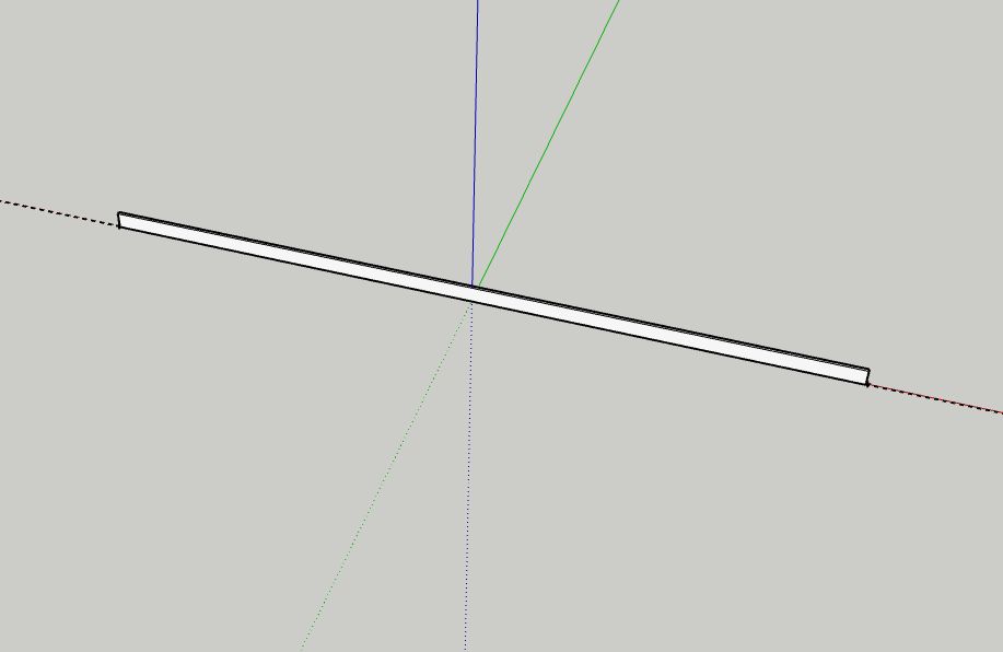
• Include at the back (250m) a small (dummy) box (which is needed for being able to simulate things in CFD)
  
• Sluit af als klaar: 'Save' en 'Download' -> 'STL'
• Effort: 0.5 hours.

Editing 3D-model in SIMSCALE

We are making use of SIMSCALE. Make sure you make a Community Plan account. This Community Plan allows only for 10 simulations (but one can do many more; but with more manual work). Anyway make sure you have a good CAD-model and that you train/educate yourself around SIMSCALE.
The following steps can be done:

• Het simulatie project staat hier.
  
• Import het STL model
• Edit this (not yet rotated) model by: Edit a copy
  
• Make a Flow Volume -> External waarbij de poreuze objecten (bomen: 'Excluded parts') niet deelnemen aan het 'External flow volume'.
  
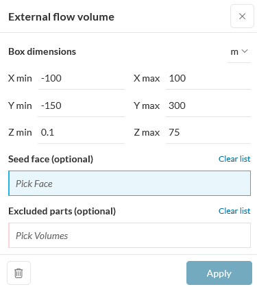
  Zie voor richtlijnen mbt vrije afstanden rondom het model hier [Franke, 2007]:
  
  • Xmin, Xmax: minimaal 5*hoogte/grootte hoogste obstakel [Franke, 2007, page 17] extra aan linker en rechter kant van 3D-model. In dit geval ~5*~20m (molen): ~ 150m
  • Ymin: Distance in front of model (in Y-direction) minimaal 8*hoogte/grootte hoogste obstakel [Franke, 2007, page 18] extra aan voorkant van 3D-model. In dit geval ~8*~20m (molen): ~ 150m
  • Ymax: Distance at back of model (in Y-direction) minimaal 15*hoogte/grootte hoogste obstakel [Franke, 2007, page 18] extra aan achterkant van 3D-model. In dit geval ~15*~20m (molen): ~ 300m
  • Zmin: Ground (in Z-direction) minimaal om invloed van modelerings afrondingen te voorkomen:  ~ 0.1m
  • Zmax: Height (in Z-direction) minimaal 6*hoogte/grootte hoogste obstakel [Franke, 2007, page 17]. In dit geval ~6*~20m (molen): ~ 150m
  • By the way, the default values in SIMSCALE were always somewhat larger than the above, so its defaults are also ok. Except for Zmin; I would put that always at 0.1m.
    
• Delete the dummy box, maar niet de fence
  
• Save
• Effort: 0.5 hours.

Configureren van de CFD

Take the following steps (if not default, it is explicitly mentioned in below steps):
<the screen grabs are not fully matching the text: the text is leading>

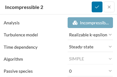
• Goto SIMULATIONS +
• Incompressible -> Turbulence-model -> Realizable k-epsilon [Franke, 2007, page 14]
  
  
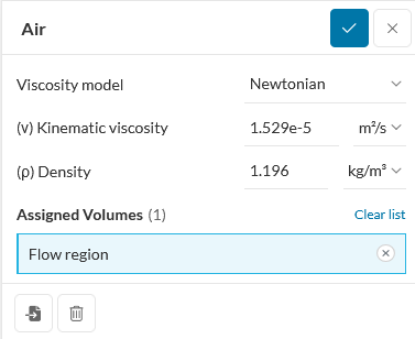
• Materials -> Air -> Apply
  Assigned Volumes -> Flow region
  
  
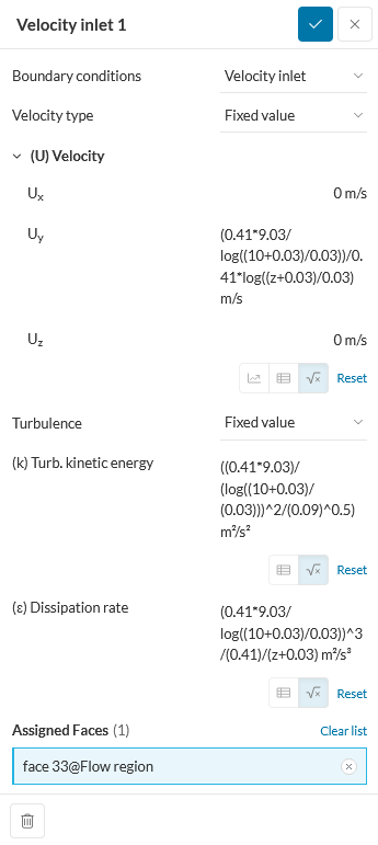
• Boundary conditions
• Velocity Inlet
  Assigned Faces -> the wind side
  (U) Velocity -> U_y -> ABL Formula (7.42m/sec at 10m and z₀=0.0132m, the wind direction is 180deg [S])
  (0.41*7.42/log((10+0.0132)/0.0132))/0.41*log((z+0.0132)/0.0132)
  Turbulence -> Fixed value
  (k) Turb. kinetic energy -> ABL derived Formula
  ((0.41*7.42)/(log((10+0.0132)/(0.0132)))^2/(0.09)^0.5)
  (ε) Dissipation rate -> ABL derived Formula
  (0.41*7.42/log((10+0.0132)/0.0132))^3/(0.41)/(z+0.0132)
  Save
  
  
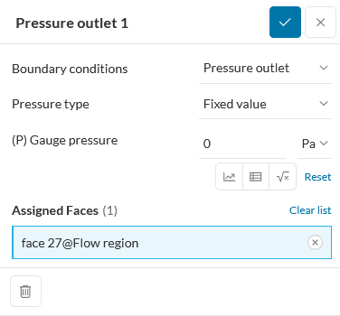
• Pressure outlet
  Assigned Faces -> opposite inlet side
  Save
  
  
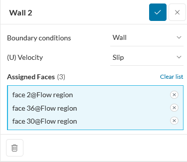
• Wall
  Assigned Faces -> two sides and top
  (U) Velocity -> Slip
  Save
  
  
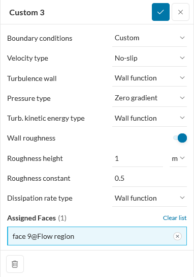
• Custom (ground)
  Assigned Faces -> bottom side
  Wall roughness -> On
  Roughness height -> 1m
  Roughness constant -> 0.5
  Save
  
  
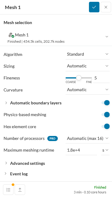
• Mesh
  25m fence: Fineness = 7.5 (1.5Mcells)
  
  
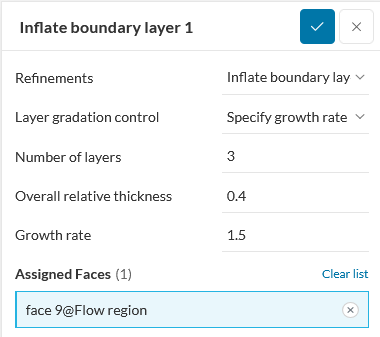
• Mesh -> Refinements -> Inflate boundary layer
  
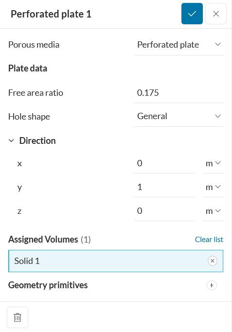
• Advanced concepts -> Porous media -> Perforated plate
  An optical porosity of 20%; this gives 8.5% for aerodynamic porosity.
  
  
• Effort: 2 hours.

Uitvoering van de CFD

• For this simulation it is handy that one can Download the results (so at least a fully functioning Community Plan). By downloading the velocity results it is easy to compare these with Tabel 4.5 to 4.8 and Figure 5.1 [Beljaars, 1979].
  
• Simulation Runs +
• Mesh size: Fineness of 7.5 has been used in below analysis.
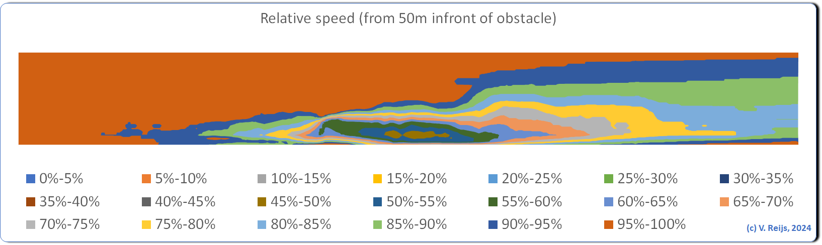
• Below is a graph of the relative speed [%]. For height from 0 to 7.5m and distance from -25m (so not -50m as stated in picture!) to ~41m. WIth aerodynamic porosity of 8.5% (Dichte Wand)
  
• Below is a graph of the relative speed [%] as simulated in CFD (continuous curves) and Beljaars (dashed curves, Tabel 4.5). For distance (x/H) from 22m (10H) to 176m (80H). And at 5 heights (z/H: 0.5H, H, 2H and 3H). WIth aerodynamic porosity of 8.5% (Dichte Wand)
  
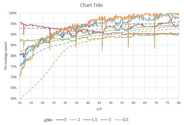
  This is slightly different behavior then seen in Beljaars (dashed curves, Tabel 4.5). All heights should (according to Townsend) go towards more or less the same percentage (94%). This migth be due to the Roughness height of ground boundarylayer in the CDF, which might influence the velocity for the long distances (x/H). Furthermore height 0.5H is quite different.
  Remark: changing this Roughness height gives no change in the CFD... What to do?
  The z/H=0.5 curve (orange dashed) of Beljaars is quite different from CFD (orange conitnous curve). This could be because Townsend's z/H=0.5 curve (used as verification of in Beljaars) is also quite different from Nägeli (which maps on the CFD). See for difference Townsend and Nägeli here.
• More to come for other z₀ and more aerodynamic porosities.
  
• Effort: 4 hours.
  

Conclusions

• Most default values of SIMSCALE look ok, except:
• Use Realizable k-epsilon
• Zmin should be always 0.1m
• The higher the Fineness the better, somewhere between 7.5 and 9 (instead of default of 5), or better: use your own mesh configuration.
  
• More to be added when more data analysis is done (for other z₀).
• It is clear that Beljaars used Nägeli to optimise Townsend's model. Nägeli's fence was porous. So Beljaars' guidelines are also mainly looking at porous obstacles.
  

References

Beljaars, A.C.M.: Windbelemmering rond windmolens. In: (1979).
Franke, Jörg  et al. COST Action 732: Best practice guideline for the CFD simulation of flows in the urban environment. Brussels, COST Office 2007.

Acknowledgements

Disclaimer and Copyright
HomeUpSearchMail