NEW
Victor Reijs' workflows by Victor Reijs
is licensed under CC BY-NC-SA 4.0![]()
![]()
![]()
![]()
Remember this web page is indicative/provisional; the findings are still under investigations, verification and trying to finalise things. So no rigths can be gotten from it;-)
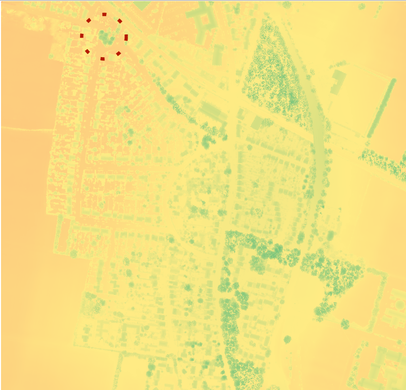
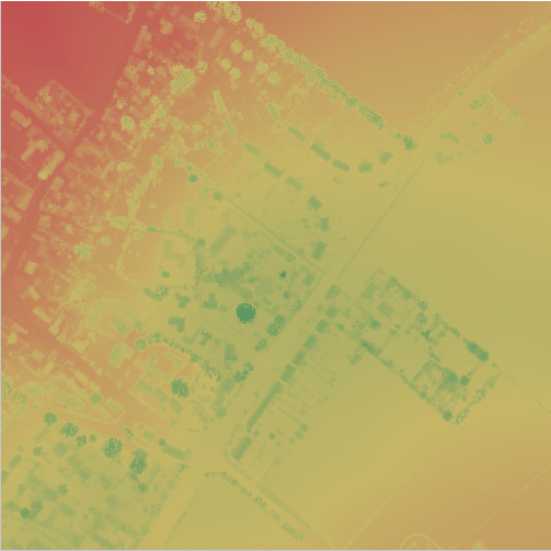
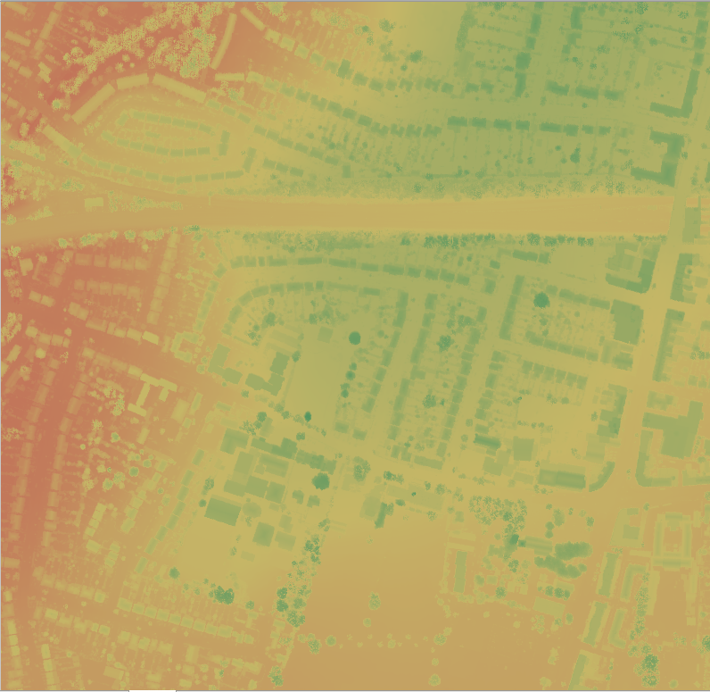
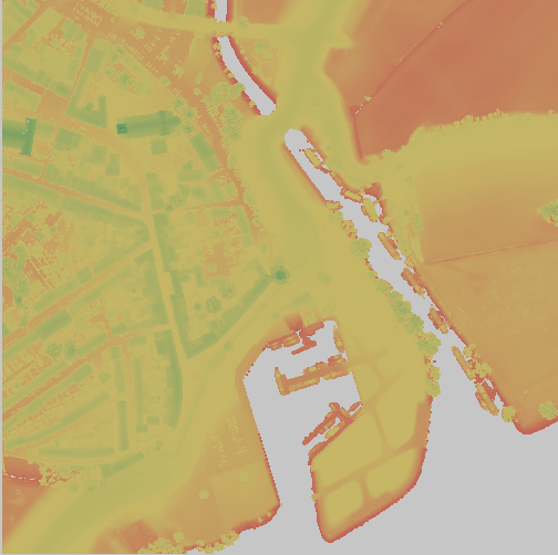
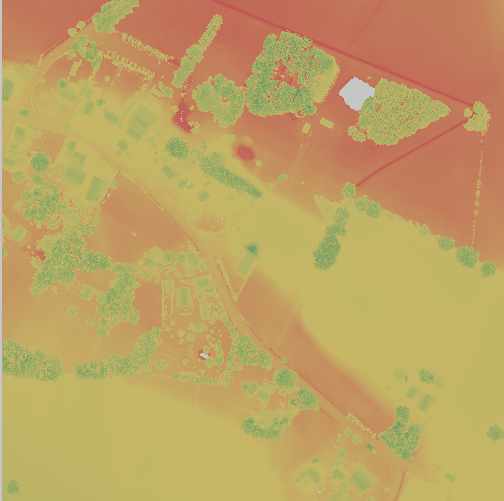
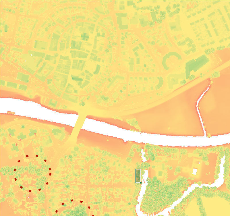
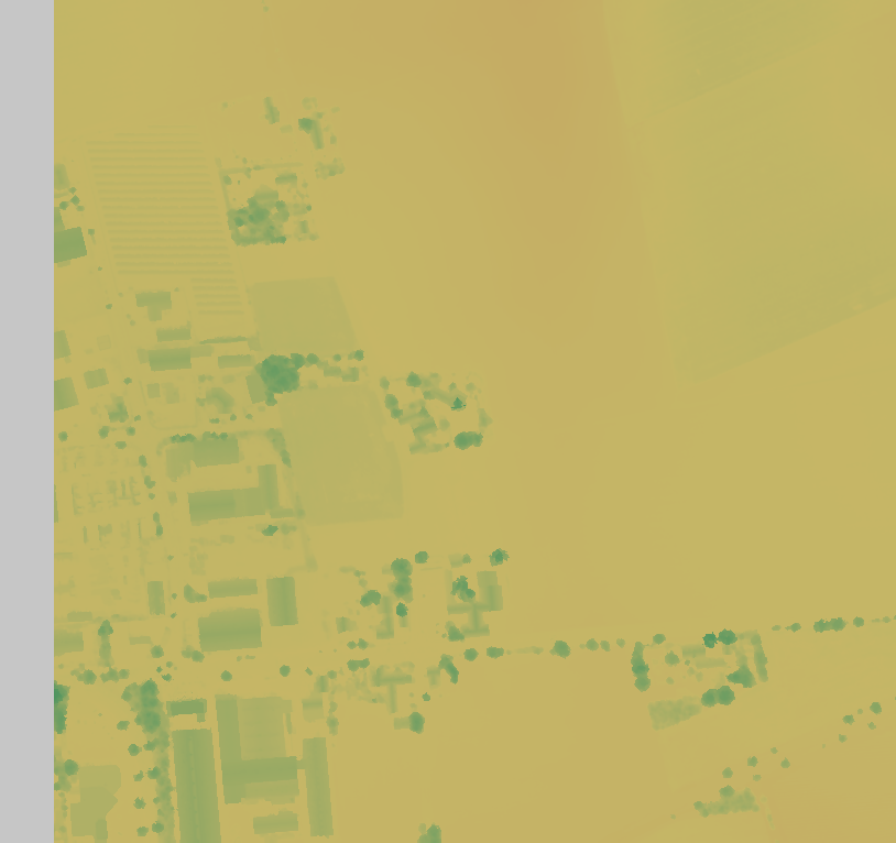
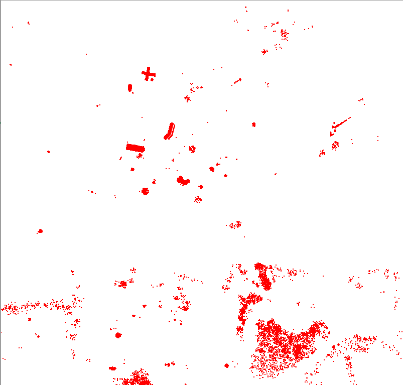
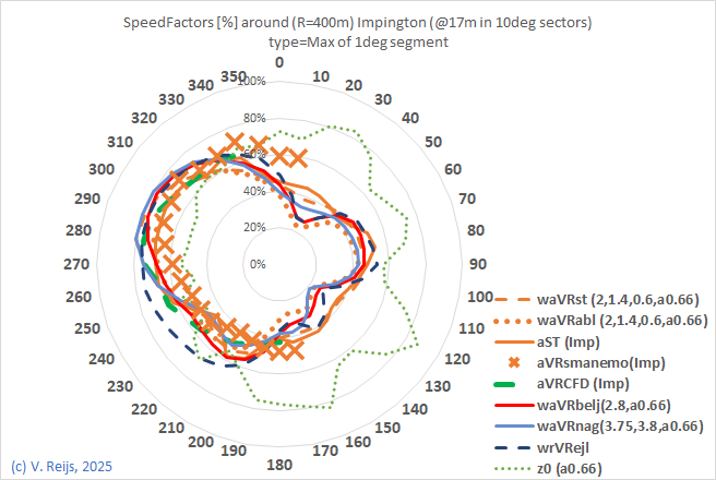
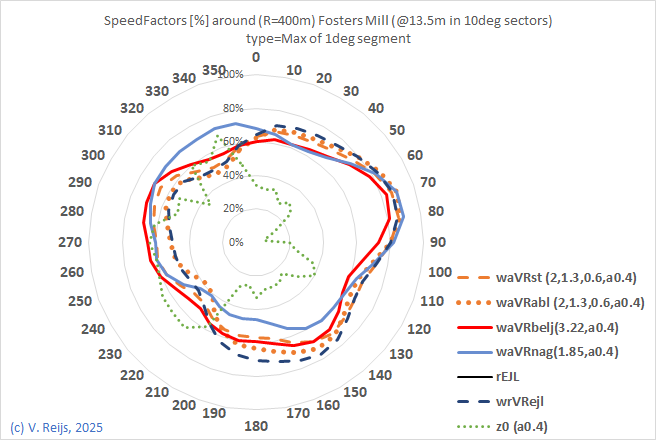
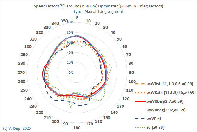
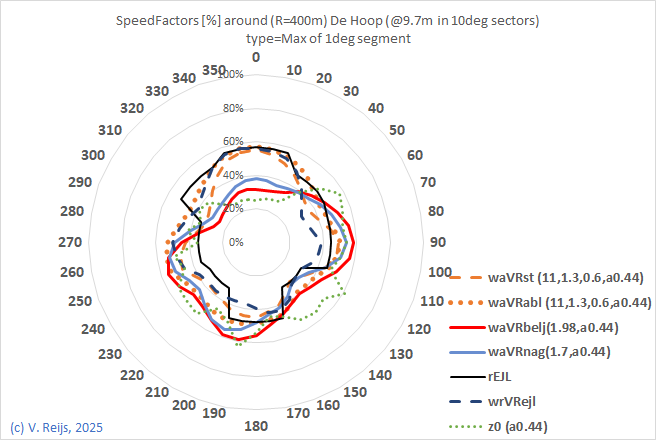
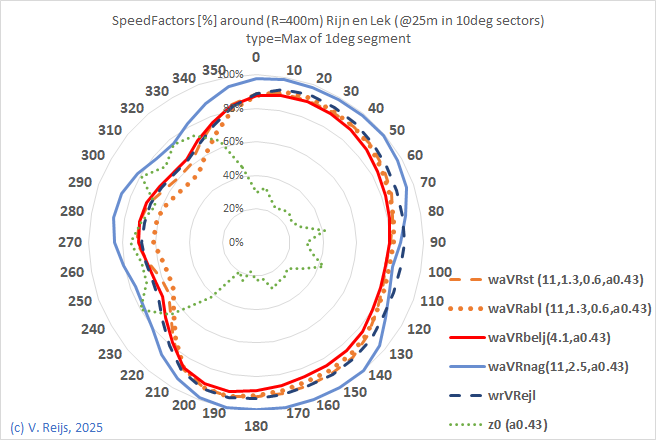
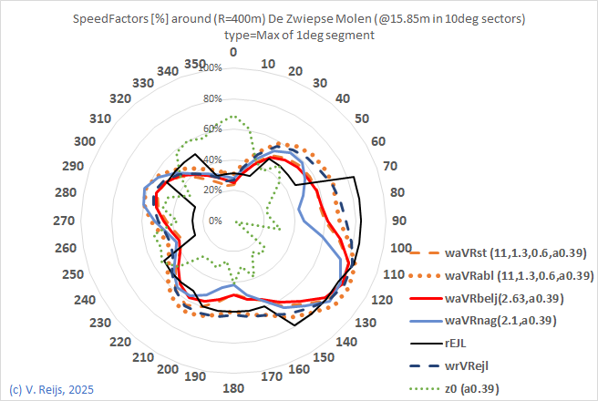
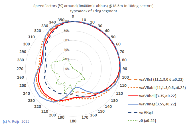
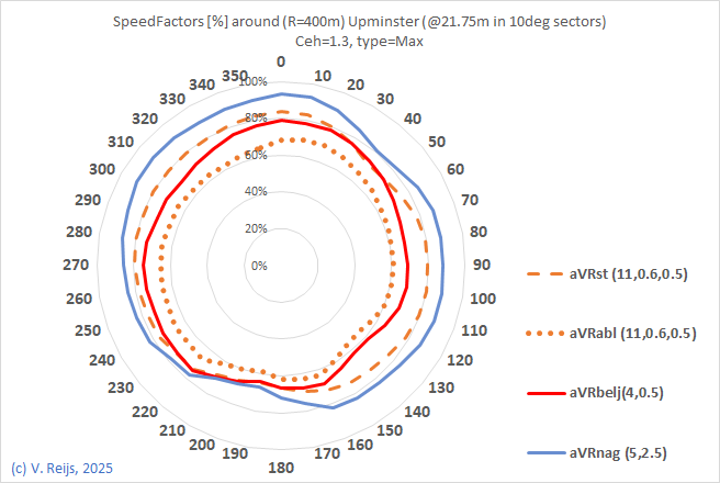
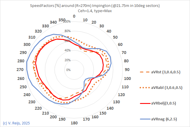
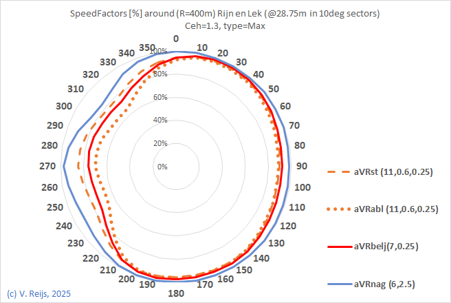
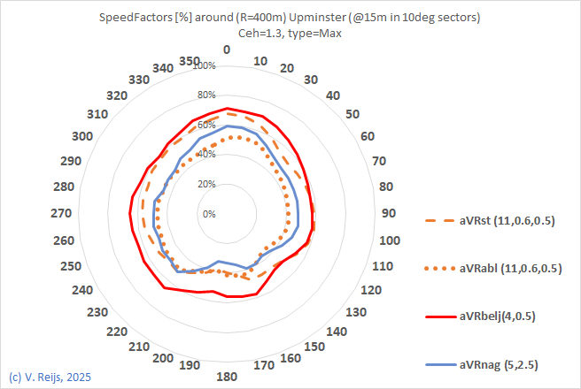
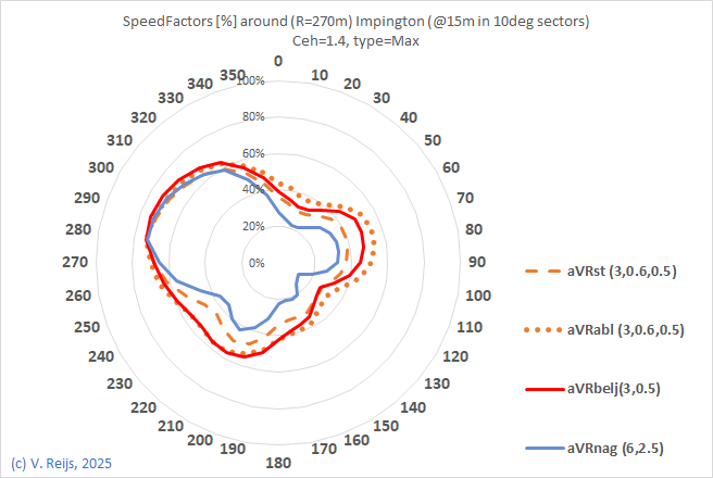
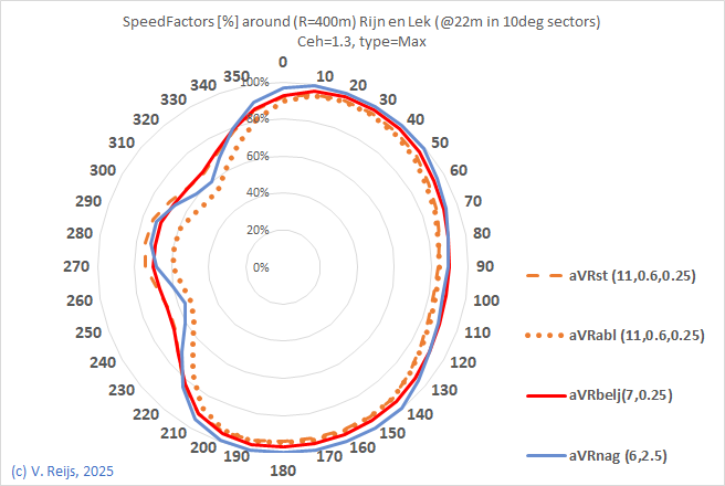
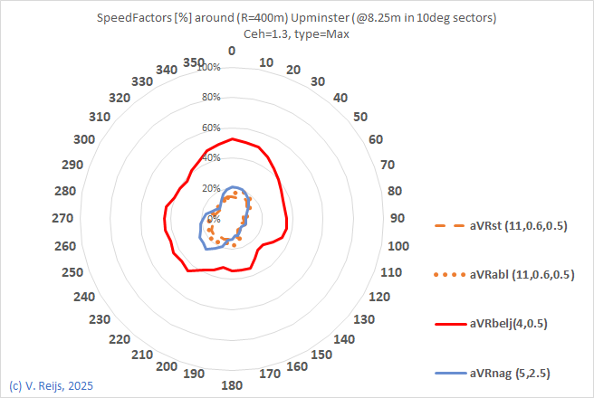
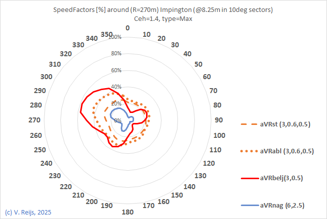
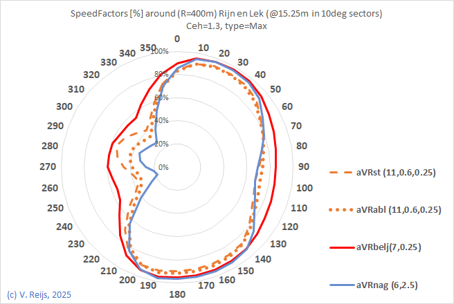
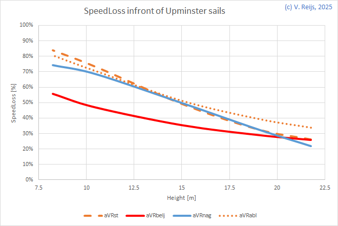
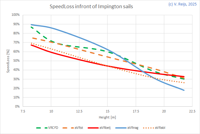
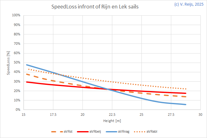
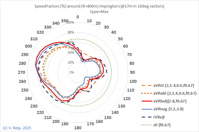
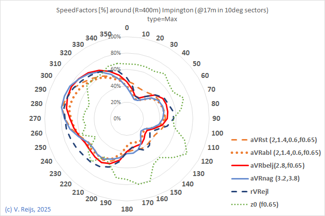
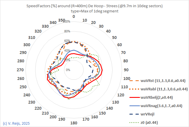
On this web page Victor Reijs' workflows are being explained, it uses a DSM around a mill (a square area with mill in the centre). It determines the obstacles (relative of the ground plain) in a speedfactor-radar of 360deg and a resolution 1deg. Five methods are being investigated: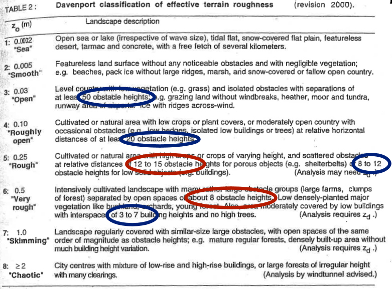
- Inspired, as a basis, by Steve Temple's method and logarithmic ABL
- From this height profile (heights are increased with an effective height factor: Ceh [called Cd by ST]), several individual obstacles are being recognised for which the Intercept height (IH) at the mill is determined (in the test environment a linear Wake decay rate of 50 is used and no distinction between house or tree). Two sub methods are used:
- aVRabl[#obstacles,Ceh,ap,z0m]
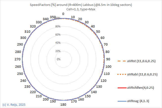
Using the obstacles' Intercept Heights (excl. Ceh), the product of speedfactor is determined by an logarithmic ABL.- aVRst[#obstacles,Ceh,ap,z0m]
Using upto 11 obstacles sorted with Intercept Heights (incl. Ceh), the speedfactor is determined using the stacking ABL function coded by Steve Temple [Temple, 2025]).- The Speedfactors of ten profiles (each of 1deg) are averaged into a (10deg) sector.
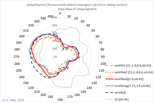
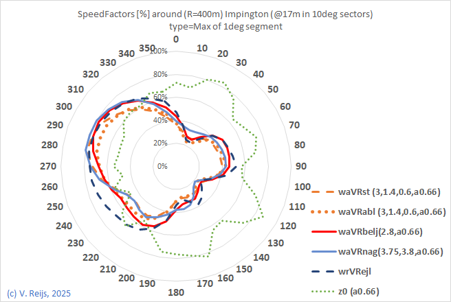
- Using, as a basis, by Evert-Jan Laméris' method (rVRejl[SF])
From this height profile, individual obstacles are being recognised for which the above HDMH height at the mill has been determined (in the test environment a linear Wake decay rate of 50 and c=0.15 is used). Adding in each 1deg profile these above HDMH heights together gives an idea of the SpeedLoss.
The lossfactor of ten profiles (each of 1deg) are averaged into a (10deg) sector. After normalising them, one can derive a kind of speedfactor (1-lossfactor/normalisation). This speedfactor is not an absolute value yet, so not 100% comparable with SpeedFactor. For comparing with other speedfactor methods, one can only look at the whole form of the curve.
- Inspired, as a basis, by VR's speedfactor formula (aVRbelj[SFmulti,z0m])
From this height profile, individual obstacles are being recognised for which the speedfactor at the mill has been determined (a variable but lineair Wake decay rate is used). The speedloss formula is derived from Beljaars tables.
The speedfactor of ten profiles (each of 1deg) are averaged into a (10deg) sector. One can derive a kind of speedfactor by multiplying each speedfactor at all distances over the radius. This speedfactor should be close to an absolute value, but the there is a Speedmultiplier (for high speedfactors = 3) which migth need alignment. So, it might not be 100% comparable with SpeedFactor, but it should be close.- Inspired, as a basis, by Nägeli (aVRnag[Cl,z0m])
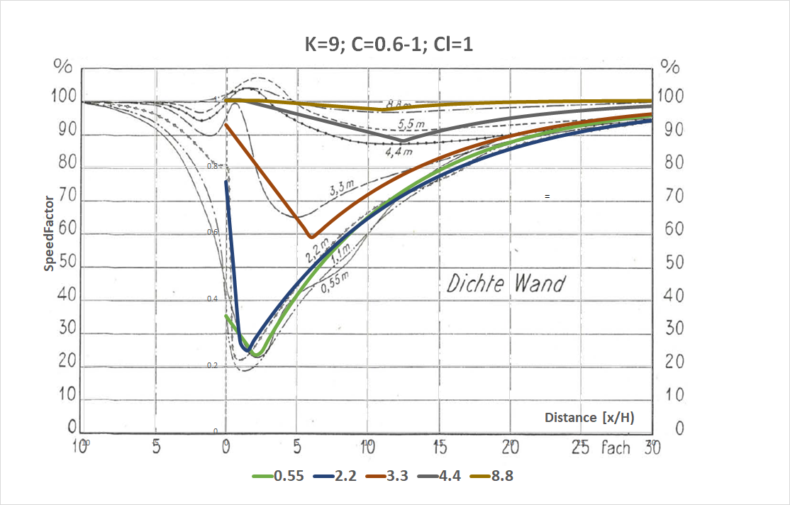
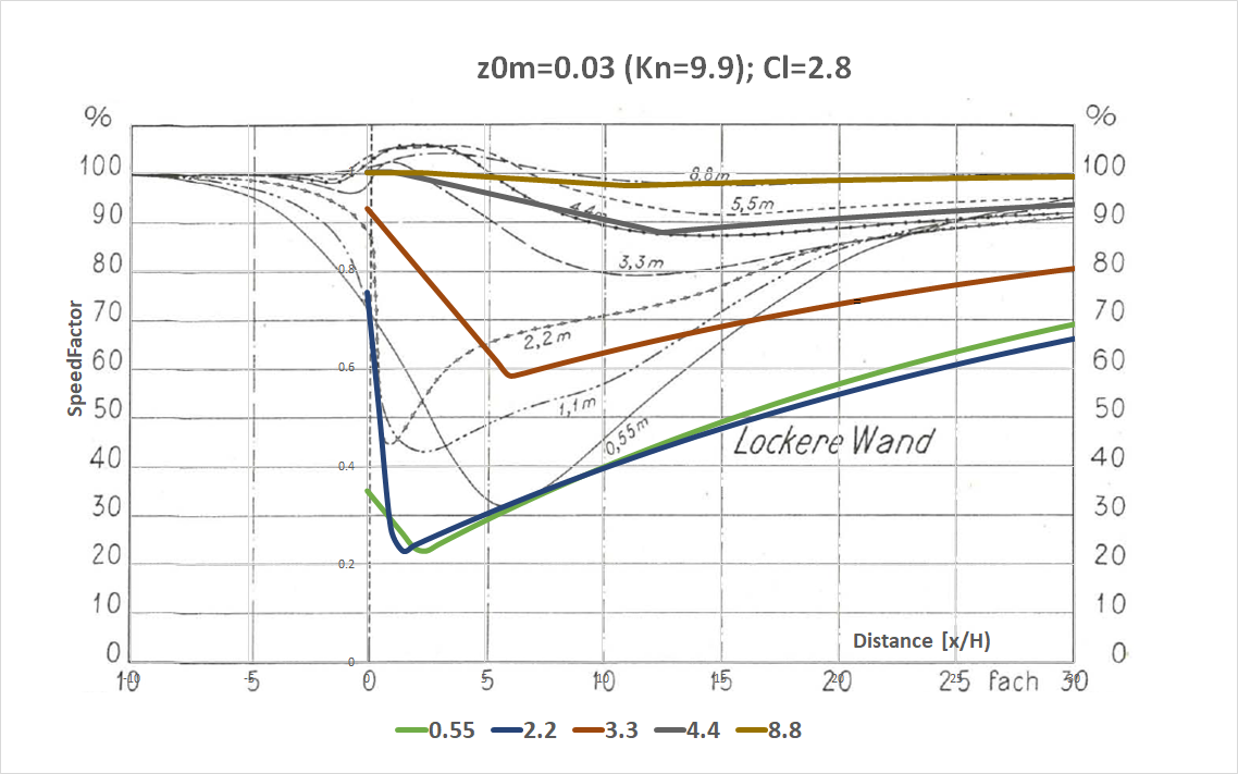
From this height profile, individual obstacles are being recognised for which the speedfactor at the mill has been determined (an exponential Wake decay rate is used). In this implementation, the SpeedFactor formula is derived from Nägeli 'Dichte Wand' (which has an optical porosity of 10-15%), by using/interpolating the below colored curves (Cl=1):
The speedfactor of ten profiles (each of 1deg) are averaged into a (10deg) sector. One can derive a kind of speedfactor by multiplying each speedfactor at all distances over the radius. This speedfactor should be close to an absolute value. It migth be that Cl needs alignment.
Nägeli is by the way independent of z0m (it has a fixed 0.03m), a factor Kn (called by EvdE: K) has been added to include this dependability.- Using, as a basis, Ezra van de Elst's method (rVRevde[z0m])
This method is based on several theories including Jensen's theory on wind turbines [1983] and Nägeli (wake behind a fence), resulting in an exponential decay of the wake.
From this height profile, individual obstacles are being recognised for which the above HEVDE height at the mill has been determined using a speedfactor =1. Adding in each 1deg profile these above HEVDE heights together gives an idea of the SpeedLoss.
The lossfactor of ten profiles (each of 1deg) are averaged into a (10deg) sector. After normalising them, one can derive a kind of speedfactor (1-lossfactor/normalisation). This speedfactor is not an absolute value yet, so not 100% comparable with SpeedFactor. For comparing with other speedfactor methods, one can only look at the whole form of the curve.
- For all methods: A weighted (using normal distribution) average is then used over five 10deg sectors. These weighting maps the normal distribution of wind directions in actual wind. The weighted average gives an idea of the Speedfactors (reduction of the wind in that sector direction).
Remark: The weighting of anemometer readings still needs some though.
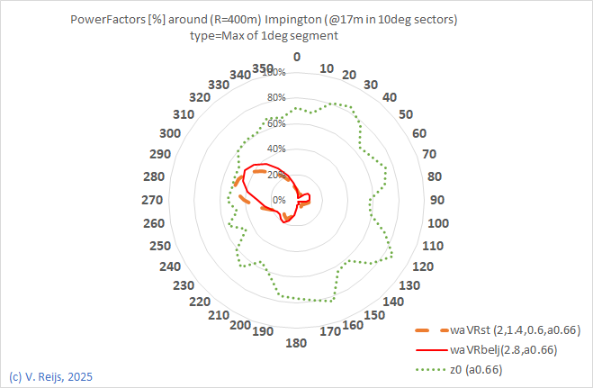
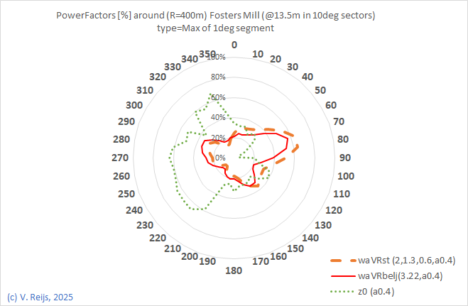
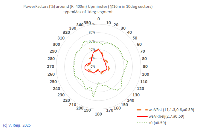
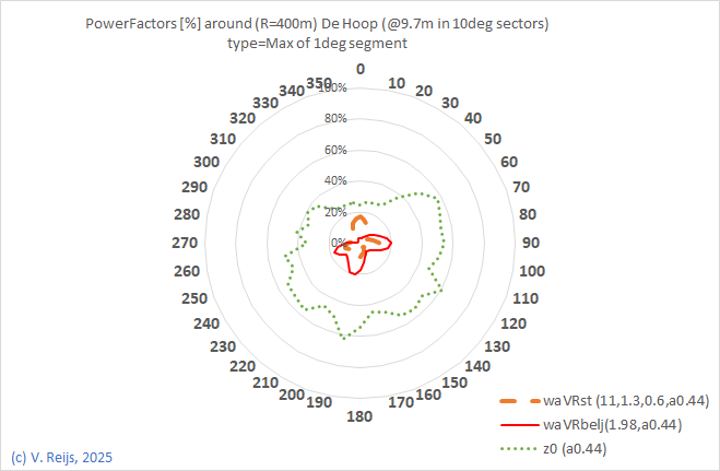
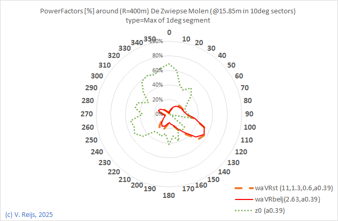
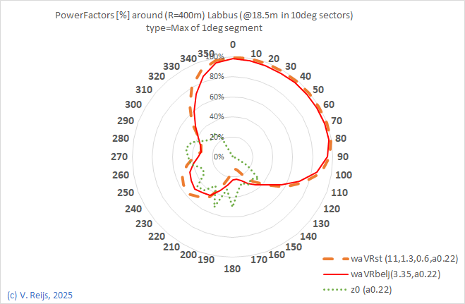
- From this the powerfactors-radar can be determined (SpeedFactor3). Both, speed and power, are presented in graphs in Excel.
Important to understand that the powerfactor-radar is not a good indication of the Effective Usable Energy (EUE: one needs to include the windrose).
- In a seperate spreadsheet an indication of the EUE (Effective Usable Energy) is given. The type of sail system determines the efficiency (Ce) of the sails.
It is important to realise that methods based/related
on the DHM formula or Beljaars tables have the following
constrains:
Trees in the neighbourhood of the mill are difficult to
simulate using DHM formula. Be aware of this!
Methods start with r(elative) are relative to something (unknown). As it are not absolute values, one could compress or enlarge (aka normalise) these curves for comparing with a(bsolute) curves.
| Method |
Based on |
Reference |
Arithmatic |
Knobs |
Ceh |
c |
wake
decay |
n |
| aST | Stacked ABLs |
Absolute |
Ceh,ap,n,z0m |
1.4 |
NA |
linear |
50 (95%) | |
| aSTanemo | wind |
Absolute |
U/Uref | scale,z0a | NA |
NA |
NA |
NA |
| aVRst | Stacked ABLs |
Absolute |
Ceh,ap,n,z0m | 1.4 |
NA |
linear | 50 (95%) | |
| aVRabl | Multiply ABLs |
Absolute |
ap,n,z0m | 1 |
NA |
linear |
50 (95%) | |
| rEJL | DHM |
Relative |
c,n,z0m | 1 |
0.2 (95%) | linear | 50 (95%) | |
| rVRejl | DHM |
Relative |
SF,n,z0m | 1 |
0.2 (95%) |
linear | 50 (95%) | |
| aVRbelj | Inverse DHM |
Absolute |
SFmulti,n,z0m | 1 |
(1-SpeedFactor)*3 |
log function on H/z0m | depending on H/z0m
(95%) |
|
| aVRevde |
exp |
Relative |
z0m | 1 |
NA |
exponential |
NA |
|
| aVRsmanemo | wind |
Absolute |
U/Uref |
scale,z0a | NA |
NA |
NA |
NA |
| aVRCFD | simulation |
Absolute |
RANS | many |
NA |
NA |
NA |
NA |
| aAEGMCFD |
simulation | Absolute |
RANS | many | NA |
NA |
NA |
NA |
| aVRnag |
exp |
Absolute |
Cl,z0m | 1 |
NA |
SF(0), SFmin
and SF(X)=linear and exponential |
NA |
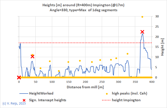
| Impington,
UK |
Fosters
Mill, UK |
Upminster,
UK |
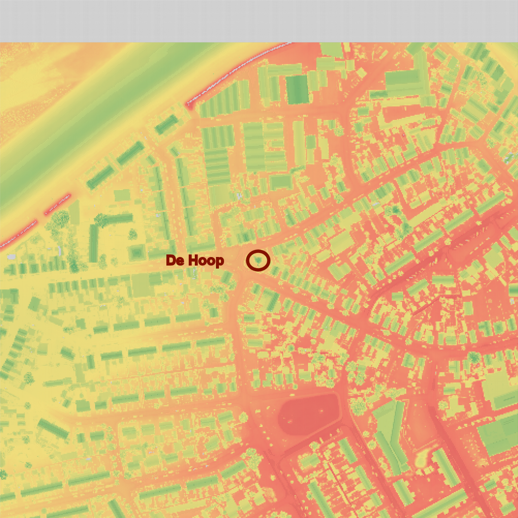
De
Hoop, NL |
Rijn
en Lek, NL |
De
Zwiepse Molen, NL |
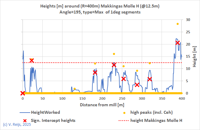
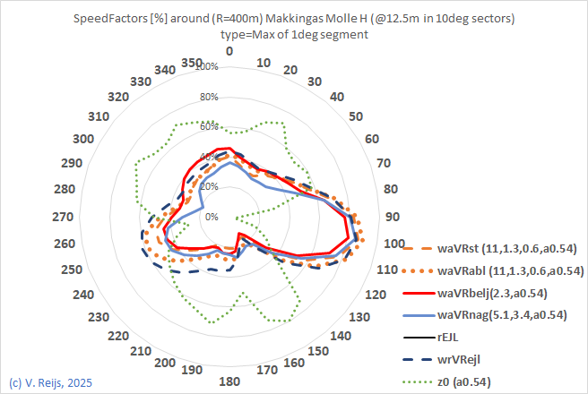
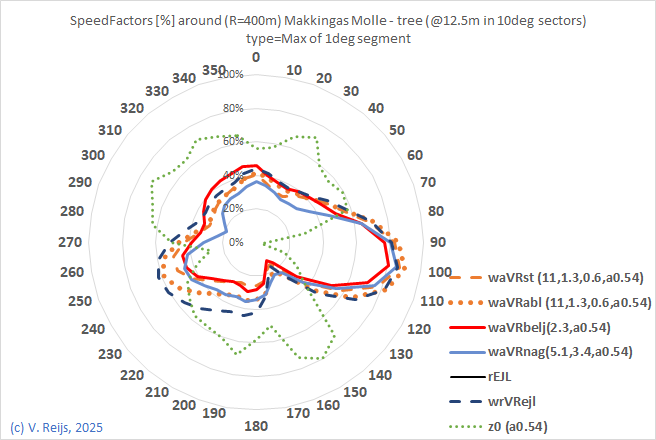
Makkinga’s
Mölle |
Labbus,
DE |
|
| DSM |
 |
 |
 |
 |
 |
 |
 |
 |
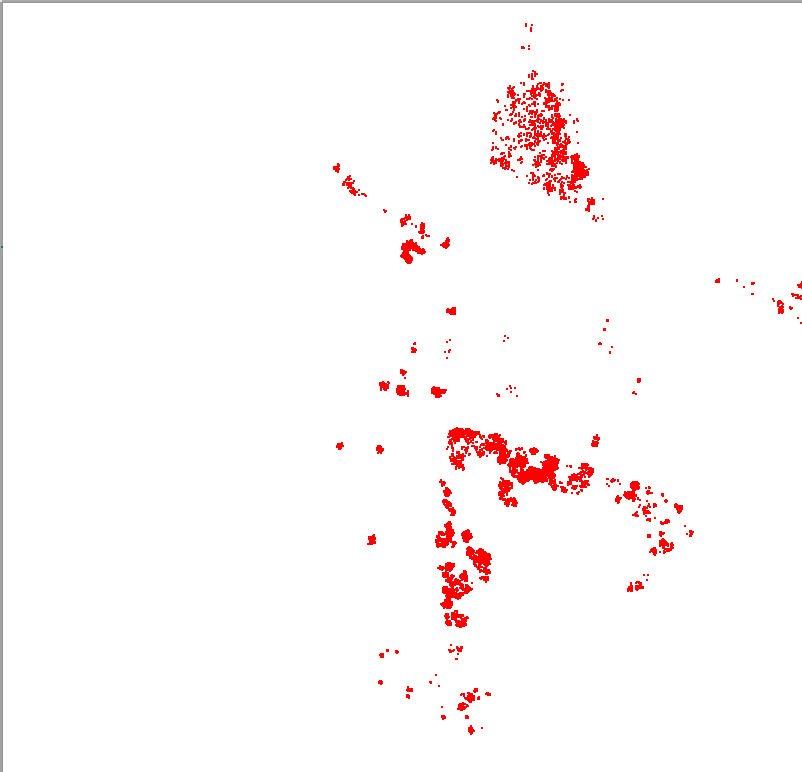
| Intercept
height > Mill height |
 |
 |
||||||
| Size
DSM |
800*800m |
500*500m aSTanemo measurements are in wintertime |
800*800m |
500*500m |
500*500m |
500*500m |
800*800m |
800*800m |
| Impington,
UK |
Makkinga’s
Mölle, NL |
 |
 |
| Factor |
Impington,
UK |
Fosters
Mill, UK |
Upminster,
UK |
De
Hoop, NL |
Rijn
and Lek, NL |
De
Zwiepse Molen, NL |
Labbus,
DE |
| Speed factor for 400m radius |
 |
 |
 |
 |
 |
 |
 |
| Power factor for 400m radius |
 |
 |
 |
 |
 |
 |
 |
| Remarks |
mp @ anemometer height There is an optimum by shrinking aST with 10deg; 20deg shrinking was seen when evaluating CFD against aST. |
mp @ anemometer height No shrinking angle for aST is relevant. |
mp @ anemometer height |
mp @ windshaft height rEJL data is here rEJL is based on old AHN-1 |
mp @ anemometer height | mp @ windshaft
height rEJL data is here rEJL is based on AHN-4 |
mp @ anemometer height |
| #Obstacles |
Impington,
UK |
| 11 obstacles used in aVRst |
 |
| 3 obstacles used in aVRst |
 |
| 2 obstacles used in aVRst |
|
| Height
(mp) measurement point |
Upminster,
UK |
Impington,
UK |
Rijn
en Lek, NL |
| +6.75m |
 |
 |
 |
windshaft @ 15m, 15m, 22m |
 |
 |
 |
| -6.75m |
 |
 |
 |
| All heights @ direction 235deg |
 |
 |
 |
| Impington, fixed z0m | Impington, variable z0m |
 |
 |
| Trees |
Makkinga’s
Mölle, NL |
De
Hoop, NL |
| With currrent tree(s) |
 |
|
| Without tree(s) |
 |
 |
| Remarks |
There is only a small
difference due to the 19m tree around 23m in 200deg. |
There is only a small
difference due to the some 12m high trees around 50m in SW |
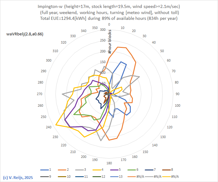
| Number
of hour blocks per sector with a certain speed |
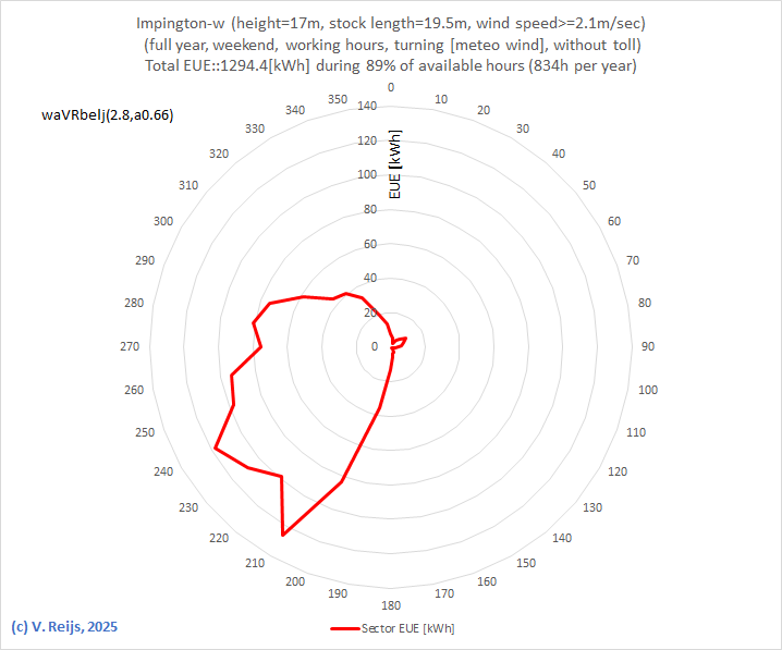
EUE
per sector |
 |
 |
| aVRst | aVRbelj | aVRabl | aVRnag |
| ap=0.6 |
SFmultiplier=2 - 4 |
ap=0.6 | Cl=1.7 - 3.8 |
| Ceh=1.4 |
Ceh=1 |
Ceh=1.4 | Ceh=1 |
Davenport, Alan G. et al.: Estimating the roughness of cities and
sheltered country. In: 12th applied climatology. 2000.
Hertwig, Denise et al.: Wake characteristics of tall buildings in
a realistic urban canopy. In: Boundary-Layer Meteorology 172
(2019), pp. 239-270.
Jensen, N.O.: A note on wind generator interaction. In: (1983),
issue RISO-M-2411.
Prinsenmolen-Committee: Research inspired by the Dutch windmills.
H. Veenman 1958.
Temple, Stephen: Mill Biotope mathematics. In: Version 5
(2025).